This appendix documents the interfaces and profiling methods used by the expert-parallel, grouped-GEMM, and MXFP8 implementations (Sections 5, 9, and 11). It records the operation boundaries, payload requirements, and measurements needed to reproduce and maintain these paths.
A.1 Rowwise Dispatch and Combine Use PUT/GET
The rowwise operation stack has four conceptual levels: model-level MoE phase, Python autograd function, Python C++/CUDA extension wrapper, and CUDA kernel using NVSHMEM PUT/GET primitives (NVIDIA 2026s, 2026r).
The phase name does not determine the transport primitive; dispatch and combine each use PUT in one direction and GET in the other:
| MoE phase | Transport | Why |
|---|---|---|
| Dispatch forward | PUT | Source-token rank holds the input row and pushes it to the rank that stores the selected expert. |
| Combine forward | GET | Source-token rank produces the combined output and pulls expert rows back. |
| Combine backward | PUT | Source-token rank pushes weighted output gradients to expert-output gradients. |
| Dispatch backward | GET | Source-token rank pulls route gradients and sums them into token gradients. |
The autograd node names below are private implementation classes and change with the code; the wrapper names are the stable interface. The BF16 separate autograd nodes are:
| Autograd node | Forward wrapper | Backward wrapper |
|---|---|---|
_DispatchRowwiseAutograd |
rowwise_dispatch_put |
rowwise_combine_get |
_RowwiseCombineWeightedAutograd |
rowwise_combine_get |
rowwise_dispatch_put |
The FP8 separate autograd nodes are:
| Autograd node | Forward wrapper | Backward wrapper |
|---|---|---|
_DispatchRowwiseFP8Autograd |
rowwise_dispatch_put_scaled |
rowwise_combine_get_scaled |
_RowwiseCombineWeightedFP8Autograd |
rowwise_combine_get_scaled |
rowwise_dispatch_put_scaled |
The fused FP8 node, _RowwiseFP8DispatchExpertsCombineAutograd, exposes the whole routed expert region as one autograd node. Its forward half covers scaled rowwise dispatch, up/gate scaled grouped GEMM, SwiGLU, down scaled grouped GEMM, and scaled rowwise combine. Its backward half runs the adjoint sequence: combine backward through scaled dispatch, down dgrad/wgrad, SwiGLU backward, up/gate dgrad/wgrad, and dispatch backward through scaled combine.
A.2 Rowwise Wrappers Enforce Runtime Requirements
The main Python wrappers are:
| Wrapper | Requirement |
|---|---|
rowwise_dispatch_put |
Push rows from local input to peer out according to dst_ranks and dst_rows; optional probs applies route weighting. |
rowwise_dispatch_put_scaled |
Quantize high-precision rows to MXFP8 qdata/scales, then PUT qdata and scales into separate peer buffers. |
rowwise_combine_get |
GET remote expert rows into local route scratch and reduce [N, K, D] into [N, D], optionally weighted by route probabilities. |
rowwise_combine_get_scaled |
GET qdata and scales, dequantize/reduce locally, and optionally save gathered routes for router-probability gradients. |
rowwise_gather_get |
One-to-one GET helper used by scaled combine and other route-gather cases. |
rowwise_combine_get_fused |
BF16/half extension path that combines GET and reduction in one CUDA kernel. |
The regular path materializes two physical route tensors, dst_ranks[N, K] and dst_rows[N, K], where N is the number of local token rows (the \(T\) of Section 5.4) and K is top-\(K\). Combine wrappers may pass those same tensors under source-oriented argument names; there are not four independent route maps.
Invalid routes use negative rank or row values. PUT kernels skip invalid routes. BF16 combine can zero-fill invalid gathered rows. FP8 scaled combine masks invalid routes before reduction.
The usual barrier defaults are:
| Operation | Pre-barrier | Post-barrier |
|---|---|---|
| Dispatch PUT | false | true |
| Combine GET | true | false |
Call sites may override these defaults when TBO, buffer reuse, or lease release order requires a different synchronization point.
A.3 CUDA/NVSHMEM Kernels Operate per Route
The rowwise CUDA implementation is route-oriented. A route id is token_row * top_k + k.
The important CUDA kernels are:
| CUDA kernel | Transport primitive | Role |
|---|---|---|
dispatchRowsPut |
nvshmemx_putmem_warp |
Unweighted row dispatch PUT. |
dispatchRowsPutWeighted |
nvshmemx_putmem_warp |
Weighted row PUT when route probabilities are supplied. |
gatherRowsGet |
nvshmemx_getmem_warp |
Gather remote rows into local route scratch. |
combineRowsReduceKernel |
local CUDA | Reduce gathered [N, K, D] into [N, D]. |
combineRowsGetKernel |
nvshmemx_getmem_warp |
Optional fused BF16/half GET plus reduce path. |
For dispatch, each route derives the source row, peer rank, and destination row, then PUTs input[src_row] into out[dst_row] on the peer. For gather/combine, each route derives the peer and source row, GETs expert_out[src_row] into local route scratch, and reduces gathered [token_row, :, :] routes into output[token_row, :].
A.4 FP8 Transport Requires Compatible Layouts
Rowwise FP8 communication carries two payload families: MXFP8 qdata and MXFP8 row scales, usually with block size 32. BF16 dispatch writes dispatch_out[capacity_rows, hidden], while FP8 dispatch writes dispatch_out_q[capacity_rows, hidden] and dispatch_out_scales[capacity_rows, hidden / block_size].
The exact scale layout depends on the consuming grouped GEMM path, not just the numerical format. Transformer Engine, for example, uses different scale layouts for communication and GEMM and swizzles between them (NVIDIA 2026w). In Olmo’s rowwise path, the received qdata and scales are passed to grouped GEMM through its prequantized-LHS interface. This reuses the quantized payload; the consumer still converts unblocked row scales to its blocked GEMM layout.
A.5 Blackwell MXFP8 Uses Block-Scaled Tensor Core MMA
Three related terms describe different levels of the MXFP8 compute path. Olmo calls PyTorch’s scaled_mm operator and requests a BF16 result. The selected device kernel implements a tiled general matrix multiplication (GEMM), including operand movement, a Tensor Core main loop, and an output epilogue. Within that main loop, the Blackwell instruction-level primitive is the fifth-generation Tensor Core matrix multiply–accumulate (MMA), exposed by the PTX tcgen05.mma family (NVIDIA 2026a, 2026u).
| Level | Term and responsibility |
|---|---|
| PyTorch operator | scaled_mm: accepts qdata and scale tensors, selects a backend, and returns the requested output dtype. |
| Device kernel | Block-scaled GEMM: tiles the matrices, moves operands and scales, runs the reduction over \(K\), and applies the output epilogue. |
| Tensor Core instruction | tcgen05.mma: computes one matrix tile update into an accumulator. |
For BF16 operands, the corresponding Blackwell instruction family uses the kind::f16 modifier. Native MXFP8 uses kind::mxf8f6f4 together with block_scale; its full PTX family includes the choice of one- or two-CTA execution:
tcgen05.mma.cta_group::{1|2}.kind::mxf8f6f4.block_scale.
For the MXFP8 case, the instruction applies the two block-scale tensors during the reduction. Its numerical operation is
\[ D_{ij} = C_{ij} + \sum_{k=0}^{K-1} \left(S^{(A)}_{i,\lfloor k/32\rfloor} A_{ik}\right) \left(S^{(B)}_{\lfloor k/32\rfloor,j} B_{kj}\right), \tag{87} \]
where each E8M0 entry in \(S^{(A)}\) or \(S^{(B)}\) scales a block of 32 consecutive E4M3 values along the GEMM-\(K\) dimension. The logical scale grids shown in Figure 47 are the operator-facing view. The Blackwell main loop stages qdata in shared memory, copies scale factors into Tensor Memory, and keeps the FP32 accumulator in Tensor Memory; the scale grids must therefore be swizzled into the blocked physical layout expected by the kernel (NVIDIA 2026u).
The raw block-scaled MMA does not directly define a BF16 result. It updates an FP32 accumulator in Tensor Memory. The GEMM epilogue reads that accumulator and converts it to the output dtype requested by scaled_mm. In the current Olmo path, that requested dtype is BF16.
A.6 Availability of Device-Side Grouped GEMM
The PyTorch source snapshot audited for this report distinguishes the public grouped-matrix-multiplication operation from the backend selected at runtime. For CUDA, the architecture gate used by the device-offset fast path admits only compute-capability major versions 9 (SM90) and 10 (SM100 family) (PyTorch Contributors 2026a). Table 41 summarizes the resulting behavior.
| PyTorch entry point | CC major 9 or 10 | Other CUDA architectures |
|---|---|---|
BF16 torch._grouped_mm |
Device-offset fast path; no offset copy to the host | Host-loop fallback; offsets are copied to the CPU before the per-group GEMMs |
Scaled torch._scaled_grouped_mm |
Architecture gate passes | Rejected by the architecture gate rather than routed to the host-loop fallback |
The BF16 fallback makes the behavioral difference explicit: it calls offs.cpu() and then launches one matrix multiplication per group (PyTorch Contributors 2026f). The fast CUDA implementation, by contrast, instantiates CUTLASS SM90 and SM100-family grouped kernels. This is a boundary of the current PyTorch integration, not evidence that SM120 lacks Tensor Core matrix multiplication. The CUTLASS source bundled with the same PyTorch snapshot contains an SM120 grouped-GEMM example (NVIDIA 2026h), and Table 21 records the SM120 mma.sync instruction family. In particular, the restriction is not a lack of “WMMA” support: WMMA is a programming interface, while the underlying matrix-instruction family differs across GPU architectures.
A.7 Common Grouped-GEMM Shapes in Training
The matrix row count seen by grouped GEMM follows the rank-local microbatch and the routing multiplicity. For \(B_\mu\) sequences of length \(L\) and top-\(K\) routing, balanced expert parallelism gives
\[ M_{\mathrm{rank}} \simeq B_\mu L K, \qquad \overline{M}_e = \frac{M_{\mathrm{rank}}}{N_{\mathrm{local}}}, \qquad N_{\mathrm{local}} = \frac{N}{M_E}. \tag{88} \]
The EP degree does not divide \(M_{\mathrm{rank}}\): an EP-MP group of size \(M_E\) contributes that many source microbatches before distributing the routed rows over the same number of destination ranks. Table 42 shows the resulting shapes for representative training configurations. Shared-expert computation is separate, and load imbalance can move an individual rank away from the balanced expectation.
| Rank-local microbatch | Expert layout | Projection | Routed rows | |||||||
| Scale | \(B_\mu\) | \(L\) | \(K\) | \(M_E\) | \(N\) | \(N_{\mathrm{local}}\) | \(d\) | \(h\) | \(M_{\mathrm{rank}}\) | \(\overline{M}_e\) |
| Small-2 | 3 | 8K | 4 | 8 | 64 | 8 | 2048 | 2560 | 96K | 12K |
| Small-3 | 4 | 4K | 8 | 8 | 64 | 8 | 2048 | 2560 | 128K | 16K |
| Small-4 | 3 | 8K | 8 | 8 | 128 | 16 | 1536 | 1536 | 192K | 12K |
| Medium-2 | 3 | 8K | 4 | 8 | 128 | 16 | 3584 | 4096 | 96K | 6K |
| Large-2 | 1 | 8K | 4 | 8 | 128 | 16 | 6144 | 8192 | 32K | 2K |
| Ultra-2 | 2 | 8K | 4 | 32 | 128 | 4 | 8192 | 10240 | 64K | 16K |
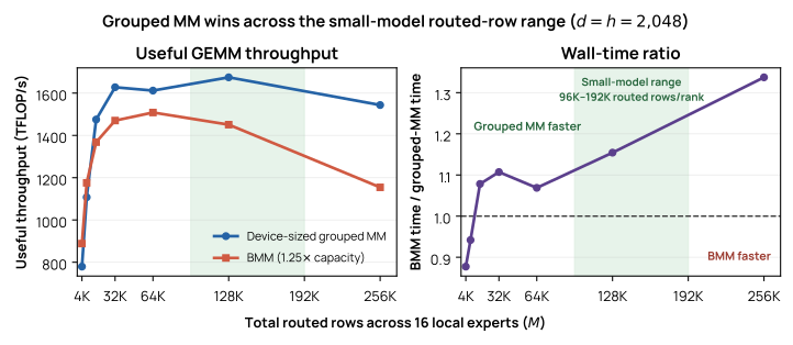
The smaller configurations in the table use expert widths between 1536 and 2560 and route 96K–192K rows per rank. To complement the \(d=h=4096\) result in the main text, we repeat the same isolated BF16 projection benchmark with \(d=h=2048\), 16 local experts, and \(M=4\mathrm{K}\) through 256K. The BMM path again executes exactly 1.25\(\times\) per-expert capacity. Its regular kernel is faster at 4K and 8K total rows; grouped GEMM becomes faster between 8K and 16K and remains faster through the rest of the sweep. At 128K total rows, BMM takes 15.4% longer.
A.8 Equal Compute Can Require More HBM Traffic
Small expert batches perform less arithmetic per weight load. A roofline model makes this limit explicit before routing, synchronization, or kernel scheduling overhead is counted. For one GPU operation, let \(F_g\) be its arithmetic work, \(Q_g\) its high-bandwidth memory (HBM) traffic, \(T_g\) its elapsed time, and \(I=F_g/Q_g\) its arithmetic intensity. With compute ceiling \(C_{\mathrm{peak}}\) and HBM bandwidth ceiling \(B_{\mathrm{HBM}}\), the idealized roofline gives (Austin et al. 2025) \[ T_g \geq \max\!\left(\frac{F_g}{C_{\mathrm{peak}}}, \frac{Q_g}{B_{\mathrm{HBM}}}\right), \qquad \frac{F_g}{T_g}\leq\min(C_{\mathrm{peak}},\,I B_{\mathrm{HBM}}). \tag{89} \] For a BF16 expert projection \([M_e,d_{\mathrm{in}}][d_{\mathrm{in}},d_{\mathrm{out}}] \to[M_e,d_{\mathrm{out}}]\), \(M_e\) is the token-row count and \(d_{\mathrm{in}},d_{\mathrm{out}}\) are the input and output widths. For this forward projection, reading both operands once from HBM and writing a BF16 result gives \[ I=\frac{2M_e d_{\mathrm{in}}d_{\mathrm{out}}} {2(M_e d_{\mathrm{in}}+d_{\mathrm{in}}d_{\mathrm{out}} +M_e d_{\mathrm{out}})}. \tag{90} \] When \(M_e\ll d_{\mathrm{in}},d_{\mathrm{out}}\), this is approximately \(M_e\) FLOP/byte: fewer rows per expert reduce weight reuse. For a stated BF16 compute reference and HBM bandwidth, the balance point is \[ I_\star=\frac{C_{\mathrm{BF16}}}{B_{\mathrm{HBM}}} \quad\text{FLOP/byte}. \tag{91} \] Under this HBM traffic model, even a zero-overhead projection below that intensity cannot reach the compute peak. Cache reuse, tiling, operand precision, and actual HBM traffic change the bound. This compute–bandwidth balance point is distinct from the measured grouped-GEMM-versus-BMM crossover in Section 9.6.
Dense and MoE forward GEMMs with equal FLOPs.
Figure 2 fixes the original token count \(T\), input width \(d\), and useful GEMM FLOPs. The dense FFN has intermediate width \(Kh\); the MoE has \(N\) experts of intermediate width \(h\) and selects \(K\) per token. Assume balanced routes with every expert used, so each expert receives \(M_e=TK/N\) rows. Dense executes the fused up/gate product \([T,d][d,2Kh]\) followed, after the pointwise activation, by the down product \([T,Kh][Kh,d]\). Grouped GEMM executes \(N\) corresponding pairs with shapes \([TK/N,d][d,2h]\) and \([TK/N,h][h,d]\). Both perform \[ F_{\mathrm{up}}=4TKdh,\qquad F_{\mathrm{down}}=2TKdh, \qquad F_{\mathrm{pair}}=6TKdh. \tag{92} \] For BF16 arrays, Table 43 counts the bytes read and written by these GEMMs. The MoE inputs are separate, already-materialized route rows; the writes that created them are outside this accounting. The down GEMM writes \(TK\) output rows before combine, whereas dense writes \(T\); combine is not folded into these GEMM writes.
| HBM traffic category | Dense bytes | MoE bytes | MoE / dense |
|---|---|---|---|
| Weight reads | \(6Kdh\) | \(6Ndh\) | \(N/K\) |
| FFN input reads | \(2Td\) | \(2TKd\) | \(K\) |
| Output writes, before combine | \(2Td\) | \(2TKd\) | \(K\) |
| Up/gate writes + down input reads | \(6TKh\) | \(6TKh\) | \(1\) |
The equal last-row count follows from the matched-compute widths, not from eliminating MoE intermediates. Dense produces \([T,2Kh]\) up/gate values and consumes \([T,Kh]\) activated values; the corresponding routed tensors are \([TK,2h]\) and \([TK,h]\). Each pair has equal element counts. In a grad-enabled BF16 forward, both paths execute a separate SwiGLU expression between the GEMMs. Its own accesses, any temporary tensors, and cache effects are outside the GEMM-only model; tensor shapes alone do not establish measured HBM traffic.
For each layout, separate the HBM bytes of the two GEMMs: \[ \begin{aligned} Q_{\mathrm{dense,up}} &= 2(Td+2Kdh+2TKh), & Q_{\mathrm{dense,down}} &= 2(TKh+Khd+Td), \\ Q_{\mathrm{MoE,up}} &= 2(TKd+2Ndh+2TKh), & Q_{\mathrm{MoE,down}} &= 2(TKh+Nhd+TKd). \end{aligned} \tag{93} \] The two GEMM passes are sequential, so their modeled times add: \[ \widehat t=\sum_{j\in\{\mathrm{up,down}\}} \max\!\left(\frac{F_j}{C_{\mathrm{BF16}}}, \frac{Q_j}{B_{\mathrm{HBM}}}\right),\qquad \widehat R=\frac{F_{\mathrm{pair}}}{\widehat t}. \tag{94} \] The figure plots \(\widehat R/C_{\mathrm{BF16}}\) as \(T\) varies, with \(N=64\), \(K=4\), and \(d=h=4096\). It uses the nominal B300 BF16 compute-to-HBM-bandwidth ratio (NVIDIA 2026q, 2026b); the vertical axis labels the common reference as peak FLOPs, not an achievable kernel rate. This is a roofline expressed against token count rather than arithmetic intensity. The hardware reference is identical; the different HBM byte counts produce different curves. At small batches, weight reads dominate and MoE reuses each weight across only \(TK/N\) tokens instead of \(T\). Larger batches amortize those reads, and both modeled curves eventually reach the common compute ceiling for these widths.
The HBM traffic model defines the scope.
This is a single-GPU forward GEMM-pair comparison, not the complete FFN or training step. Balanced, all-used routing is an analytical assumption, not a guarantee for random or learned routes. Equal FLOPs do not imply equal total parameter size or model quality. The model assumes no cache reuse between operand arrays and omits tiling-induced rereads; caching or fused indexed input access can reduce the counted HBM traffic, while rereads can increase it. Packing, route merging, activation functions, backward, inter-GPU communication, gradient synchronization, and optimizer work are excluded. Fusion or pipelining across the two GEMM passes can change their HBM traffic and timing. The curves are ceilings within these assumptions, not measured rates or an end-to-end MFU bound. Measured projection efficiency appears in Section 9.6.
A.9 The Maximum Load Does Not Specify the Expert Histogram
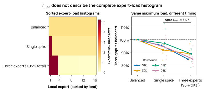
The maximum-to-mean ratio \(I_{\max}\) records only the largest expert load. It does not record how much work is concentrated among the other experts. Figure 72 constructs a direct counterexample with 16 local experts. The matched single-spike assignment gives one expert 31.67% of all rows and divides the remainder across 15 experts. The three-hot assignment gives the same number of rows to each of three experts, so those three receive approximately 95% in total and the other 13 divide the remaining 5%. After eight-row alignment, both have \(I_{\max}\approx5.07\), the same total rows, and the same useful FLOPs.
The three-hot assignment has lower mean grouped GEMM throughput at all four row counts. Its additional loss relative to the matched single spike ranges from 3 to 11 percentage points. The condition ranges overlap at some shapes, so the experiment does not make \(I_{\max}\) or any other single summary a complete timing model. It establishes the narrower point: two assignments with the same maximum load can present different collections of matrix problems to grouped GEMM and take different amounts of time.
A.10 Grouped-GEMM Capacity Benchmark Details
The benchmark in Section 9 uses 16 local experts, \(d=h=4096\), and BF16 operands. It isolates one square forward projection and compares exact device-sized grouped GEMM with BMM at \(C=\lceil\,1.25\,\overline{M}_e\,\rceil\) rows per expert. We fix capacity at 1.25 times the mean rather than the observed maximum, so balanced routes still incur the configured padding. Both paths receive the same seeded valid activations and expert weights and write into preallocated outputs. Routing, communication, activation functions, and backward are outside the timed region, so the result identifies a kernel crossover rather than predicting complete expert-MLP time.
The raw per-call timings, validation output, and manifests are retained in the experiment package bundled with this report.
A.11 Matched Grouped–Dense Projection Benchmark
This benchmark compares three mathematically equivalent BF16 projections. We initialize one canonical \(W_{\mathrm{dense}}\in\mathbb{R}^{8192\times81920}\) and partition its output columns in two ways: four expert matrices of shape \(8192\times20480\), or eight expert matrices of shape \(8192\times10240\). Both grouped layouts contain the exact dense BF16 values. One seeded input \(X\) is physically repeated for each grouped problem, and sampled output rows match bitwise at every measured \(T\).
All three paths execute \(2T\times8192\times81920\) useful FLOPs and access the same number of weight and output elements. They do not have identical input traffic: the grouped paths supply \(X\) to four or eight GEMMs. The experiment isolates this projection and excludes the activation function, down projection, routing, communication, shared experts, and backward.
We sweep powers of two from \(T=1\) through \(65536\) in eight paired trials, one on each of eight B300 GPUs. Every GPU measures both grouped partitions and their corresponding dense controls; partition order and backend order are counterbalanced. After ten direct warm-up calls, calibration chooses an adaptive CUDA Graph work unit targeting approximately 100 ms per replay. Each backend then receives a three-second pilot and a final batch containing at least eight seconds of uninterrupted same-path conditioning immediately followed by at least 1.5 seconds of measurement. The host submits both phases behind one device gate before releasing the GPU, with no synchronization or bookkeeping at the phase boundary.
| \(T\) | Dense | 4 experts | 4 / dense | 8 experts | 8 / dense |
|---|---|---|---|---|---|
| 1 | 7 | 4 | 0.588 | 4 | 0.620 |
| 16 | 111 | 67 | 0.601 | 68 | 0.608 |
| 128 | 854 | 520 | 0.608 | 548 | 0.643 |
| 256 | 1126 | 1086 | 0.964 | 1085 | 0.963 |
| 512 | 1293 | 1236 | 0.956 | 1230 | 0.951 |
| 1024 | 1381 | 1306 | 0.945 | 1298 | 0.941 |
| 2048 | 1422 | 1356 | 0.953 | 1350 | 0.949 |
| 4096 | 1401 | 1335 | 0.953 | 1331 | 0.950 |
| 8192 | 1416 | 1252 | 0.884 | 1250 | 0.882 |
| 16384 | 1412 | 1186 | 0.840 | 1184 | 0.839 |
| 32768 | 1413 | 1168 | 0.827 | 1169 | 0.827 |
| 65536 | 1411 | 1167 | 0.827 | 1167 | 0.827 |
Both grouped layouts approach the dense projection at \(T=256\) and sustain roughly 94–96% of dense throughput through \(T=4096\). Their close agreement shows that dividing the fixed projection into eight half-width GEMMs adds little cost beyond the four-way partition in this range. At 32K and 64K, all paths operate under the software power limit and grouped throughput settles at approximately 82.7% of dense, or 1.17 versus 1.41 PFLOP/s. These oversized cases diagnose large-matrix behavior; they are not representative training shapes.
A.12 Very Large Grouped GEMMs Enter a Power-Limited Clock Regime
The main sweep stops at \(M=128\mathrm{K}\) total rows, or \(M_e=8\mathrm{K}\) rows per local expert. We separately stress-tested \(M_e=4\mathrm{K}\) through \(32\mathrm{K}\), reaching 512K total rows across 16 experts. The 16K and 32K per-expert cases, 256K and 512K rows per rank across 16 local experts, are deliberately outside realistic Olmo training shapes; they expose the power-and-clock response behind the large-shape throughput decline.
The diagnostic uses eight counterbalanced trials across four B300 GPUs. Each backend and shape receives an uninterrupted three-second pilot followed by an eight-second conditioning region and a 1.5-second measured region. Shape and backend order vary across trials. The host submitted work at least 25 times faster than the GPU executed it, so CPU launch gaps were not on the measured path. All trials used BF16 operands, with expert weights drawn from a normal distribution with standard deviation 0.02 and standard-normal activations from fixed seeds, and grouped GEMM and BMM received identical valid activations and expert weights.
Figure 73 shows the relevant comparison. From \(M_e=4\mathrm{K}\) to \(32\mathrm{K}\), median grouped GEMM throughput falls from 1366 to 1163 TFLOP/s while its median SM clock falls from 1174 to 960 MHz. Per-trial useful throughput per MHz (each trial’s throughput divided by its mean SM clock) has per-shape medians between 1.16 and 1.19 TFLOP/s/MHz; dividing the median throughput by the median clock instead gives 1.16–1.21 TFLOP/s/MHz. The equal-FLOP dense control remains approximately flat at 1.41–1.42 PFLOP/s, and the unplotted capacity-BMM control remains approximately flat at 1.21–1.22 PFLOP/s. Under this sustained load, BMM takes about 6% longer than grouped GEMM at \(M_e=8\mathrm{K}\), compared with 28.9% in the short timed runs of Figure 38, and it is faster than grouped GEMM at \(16\mathrm{K}\) and \(32\mathrm{K}\).
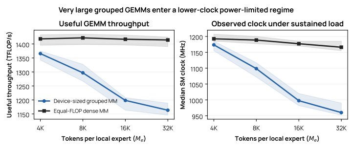
Nsight timelines at \(M_e=2\mathrm{K}\) and \(32\mathrm{K}\), captured in a separate profiling run of the same 16-expert projection, show the same CUTLASS grouped-GEMM kernel template. Together with the nearly constant throughput per MHz, this rules out a high-\(M_e\) dispatch change and provides no evidence of an algorithmic scaling collapse. Instead, sustained very-large grouped GEMMs settle at a lower clock while operating near the 1.1 kW board power limit. The precise microarchitectural reason for this lower operating point is not established. These extreme-shape timings need to be interpreted alongside clocks, power, and operand values.
A.13 Grouped Kernels Accept Managed Buffers
The BF16 grouped GEMM wrapper accepts explicit buffers:
grouped_mm(
  mat_a,
  mat_b,
  offs=expert_offsets,
  out=optional_forward_output,
  input_grad_out=optional_dgrad_output,
)
The explicit out and input_grad_out buffers matter because expert compute often writes into buffers whose reuse point is chosen by the MoE runtime rather than by the PyTorch allocator.
The MXFP8 grouped GEMM wrapper has two important forms:
scaled_grouped_mm_q(
  mat_a,
  mat_b,
  offs=expert_offsets,
  prequantized_lhs=optional_lhs_q_scales,
  prequantized_rhs=optional_rhs_q_scales,
  prequantized_rhs_for_dgrad=optional_transposed_rhs_q_scales,
)
and:
scaled_grouped_mm_q_fp8_weight(
  mat_a,
  grad_anchor,
  offs=expert_offsets,
  prequantized_lhs=optional_lhs_q_scales,
  prequantized_rhs=required_rhs_q_scales,
  prequantized_rhs_for_dgrad=required_transposed_rhs_q_scales,
  wgrad_sink=optional_fp8_weight_grad_sink,
)
Forward and dgrad can use the scaled grouped GEMM backend. Wgrad has a different current policy: the fused rowwise path dequantizes the required operands, executes BF16 F.grouped_mm, and accumulates the result into the FP8-weight gradient buffer. The integrated path has no native MXFP8 grouped Wgrad.
A.14 Fused FP8 Autograd Saves the Values Needed by Backward
The fused rowwise FP8 autograd node primarily prevents communication and expert buffers from being reused before backward finishes. When its configurable SwiGLU-recompute mode is enabled, it saves:
route maps and route probabilities
optional gathered combine routes for router-probability gradients
up_gate_q/scalesfor SwiGLU backward and BF16 SwiGLU recomputedispatched input
dispatch_out_q/scalesfor up/gate wgradgrouped GEMM offsets
In that mode, backward restores BF16 up_gate, recomputes h = swiglu(up_gate), and uses the recomputed value for down Wgrad. The configuration default enables this policy, but the production recipe explicitly disables it. Because the choice changes both retained activations and backward work, it is part of the measured workload definition.
Base-transformer recompute alternatives.
Outside the DDP stack described in Table 28, the base transformer additionally exposes module-pattern, operator-save-list, and compiler-budget modes. The operator save list always retains flash-attention outputs (Dao et al. 2022), reduce-scatter results, and the abs/max reductions reused as low-precision amax statistics, and saves every second matrix multiplication. These alternatives are separate from the DDP policies measured in Section 13.
PP and TBO composition constraint.
The pipeline schedule counts one model forward while two TBO lanes may each acquire a lease (Section 5.7). This report makes no measured claim about the slot-count factor under combined PP and TBO.
A.15 Some Kernel Prototypes Are Not Integrated
The table separates the live kernel paths from retained prototypes and identifies the conversion costs that remain in the live path.
| Boundary | Current path | Prototype or remaining cost |
|---|---|---|
| Weighted FP8 combine backward | Integrated weighting plus row quantization avoids a BF16 [N, K, D] intermediate; qdata and scales then use separate PUTs |
A direct weighted-quantize+NVSHMEM-PUT kernel exists only as an unwired benchmark prototype |
| Qdata/scale transport | Separate regular transfers in the integrated path | Paired and packed transfers are benchmark prototypes, not live training |
| Natural-layout MXFP8 grouped Wgrad | Operands dequantize and use BF16 F.grouped_mm |
Native MXFP8 grouped Wgrad exists only as a prototype; this report makes no end-to-end claim about it. |
| Scale swizzling and RHS prequantization | FP8 reduces payload size but adds separate quantization and scale-layout time, which can dominate small profiles | An RHS cache amortizes only the weight-side conversion; activation-side quantization and layout recur every microbatch |
A.16 Kernel Profiles Separate Transport and Compute Costs
Kernel profiles are interpreted through the following quantities:
| Measurement | Why it matters |
|---|---|
| Kernel launch count per MoE block | Shows whether fusion reduces Python/autograd fragmentation. |
| Dispatch PUT time | Measures route-indexed one-sided send cost. |
| Gather GET time | Measures remote row pull cost during combine and dispatch backward. |
| Combine reduce time | Separates transport from local weighted reduction. |
| Grouped GEMM time and achieved utilization | Identifies whether expert compute or communication dominates. |
| Padding/capacity overhead | Captures wasted grouped GEMM work from routing imbalance. |
| FP8 quantization time | Shows whether reduced communication payload offsets quantization cost. |
| Scale swizzle/layout time | Detects hidden FP8 layout overhead. |
| BF16 Wgrad time in the MXFP8 path | Quantifies the cost of the current non-native MXFP8 Wgrad policy. |
| Peak allocated memory by phase | Connects kernel behavior to lease high-water and PP/recompute pressure. |
| Rowwise stream wait time under TBO | Measures whether ordering waits erase overlap. |