
Routing turns one expert layer into a ragged batch of matrix multiplications. After dispatch, each rank holds token rows ordered by local expert and a device tensor containing the number of rows assigned to every expert. Grouped general matrix multiplication (grouped GEMM) executes these unequal row counts without padding every expert to a fixed capacity. A device-scheduled implementation also avoids returning the counts to the CPU.
9.1 Routing Creates Uneven GEMMs
Let \(M_e\) be the number of rows assigned to local expert \(e\), \(d\) the model dimension, and \(h\) the expert intermediate dimension. A SwiGLU expert applies
\[ \begin{aligned} U_e &= X_e W_{\mathrm{ug},e}^{\mathsf T}, & X_e &\in \mathbb{R}^{M_e\times d}, & W_{\mathrm{ug},e} &\in \mathbb{R}^{2h\times d}, \\ Y_e &= \operatorname{SwiGLU}(U_e)W_{\mathrm{down},e}, & Y_e &\in \mathbb{R}^{M_e\times d}, & W_{\mathrm{down},e} &\in \mathbb{R}^{h\times d}. \end{aligned} \tag{13} \]
Within one routed layer, every expert has the same weight shapes; routing changes only \(M_e\). The rank therefore receives \(M=\sum_e M_e\) useful rows but must execute a collection of GEMMs whose first dimension varies by expert. A single dense GEMM cannot select a different weight matrix for each segment, while launching every expert independently creates a long sequence of small operations.
9.2 Padding, Host Scheduling, and Device Scheduling
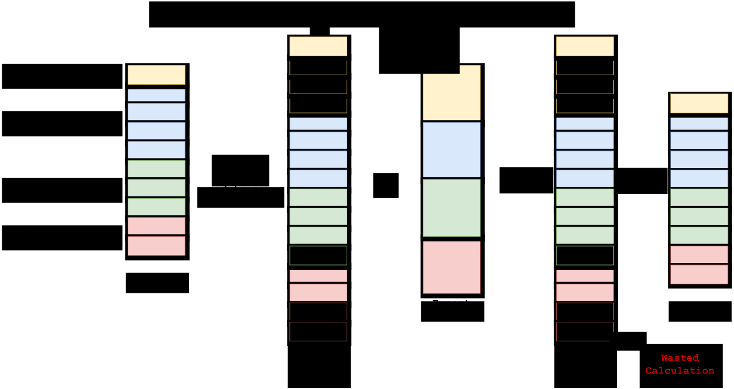
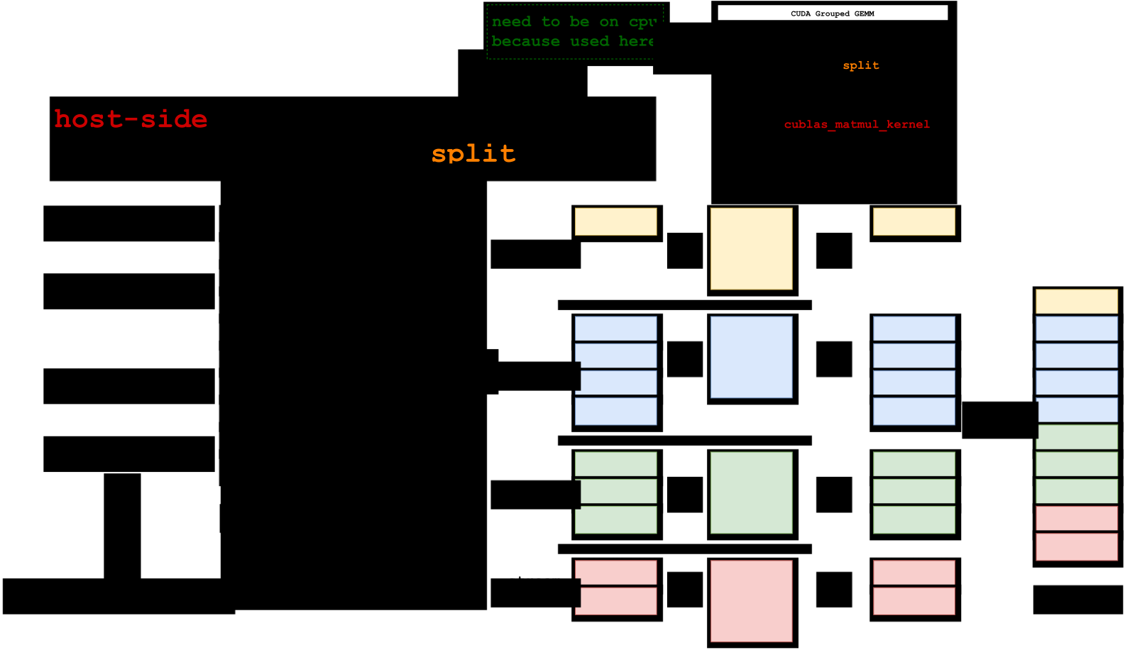
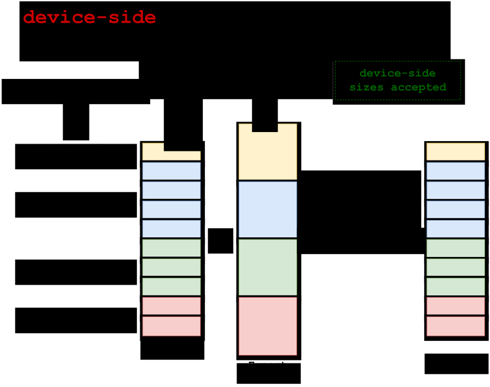
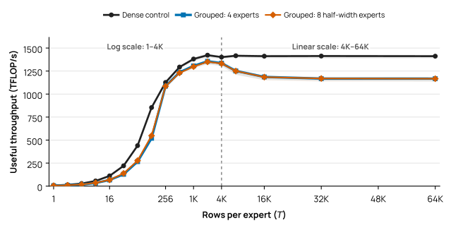
Figures 35, 36, and 37 compare three ways to execute the same expert projections. They differ in whether they pad the ragged row dimension, make its sizes visible to the host, or schedule the variable-size problems directly from device metadata.
Padded BMM.
The simplest strategy pads every expert to a common capacity \(C\) and forms an \(N_{\mathrm{local}}\times C\times d\) activation tensor. Batched matrix multiplication (BMM) then launches one regular operation, but it executes \(N_{\mathrm{local}}C\) rows even though only \(M\) rows contain routes. Its padding fraction is \[ \rho_{\mathrm{pad}} = 1 - \frac{\sum_e M_e}{N_{\mathrm{local}}C}. \tag{14} \]
The cost rises with reserved capacity and, once experts overflow their reserved rows, with load imbalance. Empty rows consume the same matrix-multiply work as routed rows.
Figure 35Interactive · conceptual mechanism, four experts · illustrative row counts
Pad every expert to capacity C, then run one regular batched GEMM
Routed rowsM = 10
Padded tokensN·C = 16 rows
Expert weightsfixed shape
Padded output16 rows
Output10 rows
Padding fraction Equation 14
ρpad = 1 − ΣMe / (Nlocal · C)
= 1 − 10 / (4 × 4) = 37.5%
- Rows multiplied
- 16
- Routed rows that fit
- 10
- Padding rows
- 6
- Capacity · sweep rule
- C = ⌈c·M̄⌉ = ⌈1.25 × 2.5⌉ = 4
Mean load M̄ = 2.5 rows per expert. Every padding row costs the same matrix-multiply work as a routed row; its output is discarded.
- Routed row (one colour per expert)
- Padding row
- Wasted output row
- Routed row beyond C
A toy layout with four local experts and one row per routed token. The routes start from the report drawing’s example (1, 4, 3, 2 rows) and the colours follow the drawing. Point at or tab to an expert to trace its rows. Changing the routes here also changes Figure 36 and Figure 37. Compare all three executions
Original report figure
Host-scheduled variable GEMMs.
An exact-size alternative makes \((M_1,\ldots,M_{N_{\mathrm{local}}})\) visible to the CPU and launches the corresponding GEMMs from a host loop. This avoids padded arithmetic, but it introduces a device-to-host dependency before expert compute can be submitted and replaces the single grouped kernel with a sequence of smaller launches.
Figure 36Interactive · conceptual timeline, illustrative block lengths · not measured
The host must read the counts before it can launch each expert GEMM
- Route + count rows
- Copy counts to the host
- CPU waits
- Launch an expert GEMM
- Expert GEMM
- GPU idle
CUDA grouped GEMM · from the report drawing
grouped_gemm( x , w , split ) = y# host-side sizes
for i in NUM_EXPERT:
    x_pointer = ...
    x_len = split[i]
    w_pointer = ...
    w_len = EXPERT_SIZE
    out_pointer = ...
    cublas_matmul_kernel(
        x_pointer, x_len,
        w_pointer, w_len,
        out_pointer
    )
split: need to be on cpu because used here
Host copy of split
1432
All 4 expert GEMMs are submitted.
GEMMs submitted
4 of 4
Drag across the timeline, or focus the slider and use the arrow keys to step from one event to the next. Figure 38 omits the host loop because CUDA events do not capture the preceding host wait; Section 8.4 explains the submission bubble. Compare all three executions
Original report figure
Device-scheduled grouped GEMM.
A device-scheduled backend keeps the cumulative expert offsets on the GPU. A GPU preparation kernel derives the per-expert pointers, strides, and matrix dimensions; one CUTLASS grouped kernel then schedules tiles across that problem list (NVIDIA 2026i). The current Olmo BF16 path reaches this mechanism through PyTorch grouped matrix multiplication on its CUDA fast path. MegaBlocks instead expresses expert compute as block-sparse matrix multiplication over a block-compressed layout. This avoids padding every expert to a common capacity, although its published implementation still pads each expert batch to a multiple of 128 rows for block alignment. It is a related, but distinct, execution strategy (Gale et al. 2023).
Figure 37Interactive · conceptual mechanism, illustrative rows and toy tiles
Offsets stay on the GPU; one grouped kernel computes only the routed rows
1 · GPU
Route counts
- E01
- E14
- E23
- E32
batchsize_per_expert, a device tensor
2 · GPU
Cumulative offsets
- E01
- E15
- E28
- E310
Prefix sum on the device: each value ends one expert’s segment
3 · GPU preparation kernel
Problem list
E0x[0:1]1 × d · W₀
E1x[1:5]4 × d · W₁
E2x[5:8]3 × d · W₂
E3x[8:10]2 × d · W₃
Pointers, strides and matrix sizes per expert
4 · One CUTLASS grouped kernel
Tiles across all problems
12 toy tiles · thread blocks take tiles in turn
Fixed-shape dispatch buffer · 24 reserved rows, the same shape for every routing decision
row 0final offset 1024
computed: rows [0, 10)unused capacity: outside the final offset, not computed
CPU queues the offsets, the preparation kernel and the grouped GEMM, and never reads a count.
Same routes, three executions · the three figures share these routes
Padded BMMFigure 35
- Ragged rows handled by
- Padding every expert to C
- Rows multiplied
- 16 = Nlocal·C
- Expert-GEMM launches
- 1 regular batched GEMM
Host loopFigure 36
- Ragged rows handled by
- Copying the sizes to the host
- Rows multiplied
- 10 = M
- Expert-GEMM launches
- 4, one per expert
Device-scheduled grouped GEMMThis figure
- Ragged rows handled by
- Offsets kept on the GPU
- Rows multiplied
- 10 = M
- Expert-GEMM launches
- 1 grouped kernel, after a GPU preparation kernel
Point at or tab to an expert to follow it from its count to its offset, problem, tiles and buffer rows; the tile size (2 rows × 2 column blocks) and the four thread blocks are a toy choice. The rowwise path fills expert-contiguous segments of a capacity-shaped buffer (Section 9.4); the timeline view in Figure 36 shows the same call without a host wait. Device-offset availability depends on the backend (Appendix A.6).
Original report figure
9.3 Device-Side Offsets Avoid a Host Synchronization
The route histogram is produced on the GPU. If a GEMM interface requires a Python list or CPU tensor of split sizes, the CPU must wait for that histogram before it can submit the expert work. As Section 8.4 explains, this device-to-host dependency drains the queued GPU work and can expose a submission bubble after the synchronization.
Olmo instead computes cumulative expert offsets on the device and passes them to grouped matrix multiplication. The preparation and scheduling kernels can therefore be queued without the CPU interpreting any route count. The selected backend must support device offsets. A fallback that copies them to the CPU recreates the synchronization even when the call site still says grouped_mm. Appendix A.6 records the architecture-specific availability of the current device-offset fast path.
9.4 Padded Shape, Unpadded Compute
Static physical shapes are a central advantage of the rowwise path (Section 5.4). Rowwise EP reserves capacity-shaped communication buffers, so their addresses and dimensions do not change with every routing decision. The device offsets separately describe the variable amount of work for each expert. Dispatch writes the received routes directly into expert-contiguous segments, and the cumulative offsets are computed from the real \(M_e\) values. The grouped GEMM consumes only those segments; unused capacity remains outside the final offset. Changing route counts therefore does not require new allocations or new tensor shapes at the compiled boundary, yet the unused tails are not executed.
This layout also removes a local permutation between communication and expert compute. The up/gate projection reads the dispatch buffer directly, and the down projection can write directly into the buffer consumed by combine—the direct-access pattern of Figure 20b. In backward, the buffer-aware grouped GEMM wrapper can write the input gradient back into the designated dispatch-gradient storage. Thus, the rowwise path combines fixed-shape allocation with unpadded compute and avoids an additional pack–unpack pair at the grouped-GEMM boundary. Appendix A documents the explicit output-buffer interfaces.
9.5 Forward, Dgrad, and Wgrad Are Different Problems
For a grouped linear projection \(Y_e=X_eW_e\), let \(X_e\in\mathbb{R}^{M_e\times d_{\mathrm{in}}}\) and \(W_e\in\mathbb{R}^{d_{\mathrm{in}}\times d_{\mathrm{out}}}\). Backward requires the input gradient (Dgrad) and the weight gradient (Wgrad):
\[ \nabla X_e = \nabla Y_e W_e^{\mathsf T}, \qquad \nabla W_e = X_e^{\mathsf T}\nabla Y_e. \tag{15} \]
| Phase | Left operand | Right operand | Contract | Result | Role of \(M_e\) |
|---|---|---|---|---|---|
| Forward | \(X_e\,[M_e\!\times\!d_{\mathrm{in}}]\) | \(W_e\,[d_{\mathrm{in}}\!\times\!d_{\mathrm{out}}]\) | \(d_{\mathrm{in}}\) | \(Y_e\,[M_e\!\times\!d_{\mathrm{out}}]\) | Output rows |
| Dgrad | \(\nabla Y_e\,[M_e\!\times\!d_{\mathrm{out}}]\) | \(W_e^{\mathsf T}\,[d_{\mathrm{out}}\!\times\!d_{\mathrm{in}}]\) | \(d_{\mathrm{out}}\) | \(\nabla X_e\,[M_e\!\times\!d_{\mathrm{in}}]\) | Output rows |
| Wgrad | \(X_e^{\mathsf T}\,[d_{\mathrm{in}}\!\times\!M_e]\) | \(\nabla Y_e\,[M_e\!\times\!d_{\mathrm{out}}]\) | \(M_e\) | \(\nabla W_e\,[d_{\mathrm{in}}\!\times\!d_{\mathrm{out}}]\) | Contraction length |
The algebra is the same as for a dense linear layer. The difference is that a dense layer has one common token dimension, whereas a routed layer has a different \(M_e\) for every expert (Table 15). Forward and Dgrad therefore contain different numbers of output rows per expert, while Wgrad contains different contraction lengths. For the up/gate projection, \((d_{\mathrm{in}},d_{\mathrm{out}})=(d,2h)\); for the down projection, it is \((h,d)\). These differences change operand layout, tile geometry, and output buffer opportunities. A forward-only kernel result therefore cannot predict the complete training benefit.
Precision makes the distinction sharper. Olmo’s routed MXFP8 path uses scaled grouped GEMM for forward and Dgrad, while its current Wgrad path uses BF16 grouped GEMM after reconstructing the required operands. Section 11.3 explains why the natural MXFP8 Wgrad contraction is not simply another copy of the forward operation.
9.6 Rows per Expert Determine the Throughput Crossover
Grouped scheduling removes per-expert host launches and avoids BMM’s padded rows, but it does not turn many small expert matrices into one large dense matrix. Its useful geometry is set by the vector \((M_1,\ldots,M_{N_{\mathrm{local}}})\), not only by the sum \(M\). The mean \(\overline{M}=M/N_{\mathrm{local}}\) indicates how much work is available per expert, while the spread of the \(M_e\) values determines BMM padding and how evenly the grouped scheduler can distribute tiles. Small \(M_e\) also means less weight reuse, which can make memory bandwidth the limit even before scheduling overhead. Appendix A.8 derives this idealized bound; the comparisons below measure actual kernel performance.
We measure the costs of fixed capacity and of splitting one projection into expert-sized problems, then vary the expert-load histogram at fixed work. A separate stress diagnostic extends beyond the training range to investigate the decline at large shapes. We omit the host loop from the kernel-speed comparison because CUDA events do not capture the preceding host wait.
The cost of fixed capacity.
The legacy BMM path sets its per-expert capacity from the ideal mean load \(\overline{M}\) and a capacity factor \(c\). Olmo applies eight-row alignment to each source rank’s share of that load, so with \(M_E\) EP ranks
\[ C = M_E\cdot 8\left\lceil\frac{\lfloor c\,\overline{M}/M_E\rfloor}{8}\right\rceil. \tag{16} \]
For \(c=1.25\), the ideal capacity already contains 25% more rows than useful work, or a 20% padding fraction; eight-row alignment can increase that gap further.1 This is different from choosing \(C=\max_e M_e\) after observing the routes. Grouped GEMM instead uses the real cumulative counts and excludes every unused capacity row.
The crossover sits at a few hundred rows per expert.
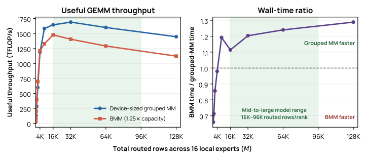
On one B300 with 16 local experts and \(d=h=4096\), Figure 38 compares one BF16 exact-row grouped expert projection with BMM at 1.25\(\times\) per-expert capacity while sweeping the total routed-row count \(M\) from 64 rows to 128K. BMM executes 25% more rows at every point, but its regular kernel is faster through \(M=4\mathrm{K}\). The crossover lies between \(M=4\mathrm{K}\) and \(M=8\mathrm{K}\), corresponding to 256–512 routed rows per expert, and grouped GEMM is faster at every measured point above it, although its advantage remains shape dependent. Avoiding padding is insufficient below the crossover, while at \(M=128\mathrm{K}\) BMM takes 28.9% longer, more than its 25% of padded work. The common mid-to-large-model operating range of 16K–96K routed rows per rank, shaded in the figure, lies entirely above the crossover. Smaller models use narrower expert projections and often place more rows on each rank, so their crossover must be measured separately; Appendix Figure 71 repeats the experiment with \(d=h=2048\), representative of that regime, and extends the routed-row sweep to 256K.
Figure 38Interactive · measured, one B300 · BF16, 16 local experts, d = h = 4096
Where exact-row grouped GEMM overtakes capacity-padded BMM
- Grouped GEMM, exact rows
- BMM, 1.25× capacity
- Mid-to-large model range 16K–96K routed rows/rank
Total routed rows across 16 local experts (M)
M = 8,192 routed rows · 512 per expert · BMM multiplies 16 × C = 16 × 640 = 10,240 rows
Plotted from the report’s sweep summary (summary.csv of the capacity sweep in the grouped-GEMM experiment package), the same values as the original figure. Appendix Figure 71 repeats the sweep with d = h = 2048. Point at, drag across, or focus a panel and use the arrow keys to read each measured point; ratios and the padded-row rate are computed from those values.
Original report figure
The cost of decomposing one projection.
To isolate decomposition, we begin with one BF16 weight \(W_{\mathrm{dense}}\in\mathbb{R}^{8192\times81920}\) and partition its output columns into \(N\in\{4,8\}\) expert matrices. For \(X\in\mathbb{R}^{T\times8192}\),
\[ W_{\mathrm{dense}} = [W_1\;W_2\;\cdots\;W_N], \qquad XW_{\mathrm{dense}} = [XW_1\;XW_2\;\cdots\;XW_N]. \tag{17} \]
All three layouts therefore execute the same \(2T\times8192\times81920\) useful FLOPs, contain the same BF16 weight elements, and produce the same output elements from the exact same BF16 values. The eight-expert case isolates the cost of dividing the same projection into more, narrower GEMMs, including the additional input reads. It is a projection benchmark, not a complete dense-versus-MoE model comparison.2 Splitting a microbatch into waves (Section 5.9) reduces \(T\) and lowers GEMM efficiency further, one ingredient of the wave-scheduling result in Section 15.2. The compared paths also use the same seeded operand distribution, since operand values can affect throughput (Section 19).
Figure 39 shows the absolute useful throughput of Equation 17. At very small \(T\), decomposing the projection is expensive: both grouped layouts deliver only about 58–65% of dense throughput through \(T=128\). Both improve sharply at \(T=256\), reaching about 96%, and remain at 94–96% through \(T=4096\). Doubling the number of expert GEMMs while halving their width changes throughput only slightly in this experiment. The larger gap is between either grouped layout and the single dense projection. At still larger \(T\), both grouped layouts drift to 83–88% of dense across \(T=8192\)–\(65{,}536\), settling at 32K and 64K in the power-limited regime examined below.
Figure 39Interactive · measured, one paired trial each · eight B300 GPUs, BF16
Same FLOPs, weights and outputs: what does splitting one projection cost?
- Dense control
- Grouped: 4 experts
- Grouped: 8 half-width experts
- Eight-GPU range
Equation 17 · same projection, three layouts
The expert weights are column blocks of one dense weight; each grouped path repeats the input X once per expert.
T = 128 rows per expert · every path does the same 2·T·8192·81920 = 0.17 TFLOP of useful work
1 × [128, 8192] @ [8192, 81920]4 × [128, 8192] @ [8192, 20480]8 × [128, 8192] @ [8192, 10240]Plotted from the report’s aggregate of the fixed-duration paired benchmark (means and eight-GPU ranges, as in the original figure). The “% of dense” view plots each GPU’s paired grouped ÷ dense ratio. Point at, drag across, or focus the chart and use the arrow keys to read every T; point at a series to highlight it.
Original report figure
Very large grouped GEMMs run at a power-limited clock.
The large-shape decline motivates a separate stress diagnostic extending to 32K rows per local expert. Its largest shapes are deliberately oversized diagnostics rather than representative training points. Across that range, grouped GEMM throughput declines together with the SM clock while useful throughput per MHz stays nearly constant. Nsight timelines from a separate profiling run show the same CUTLASS grouped-GEMM kernel template at \(M_e=2\mathrm{K}\) and \(32\mathrm{K}\), and the software power-cap limiter is active in effectively every telemetry sample near the board limit. The equal-FLOP dense control holds nearly flat throughput at a higher clock, and the capacity-padded BMM control, also nearly flat, overtakes grouped GEMM at 16K and 32K rows per expert. Together, these observations indicate a lower power-limited operating point rather than a kernel-selection change or a collapse in per-clock efficiency.
Clocks and power help interpret the extreme-shape decline; operand values can also affect throughput (Section 19). Appendix A.12 records the diagnostic protocol and complete curves.
Sensitivity to the load histogram.
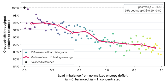
Even with total rows and arithmetic fixed, the shape of the expert-load histogram changes grouped GEMM time. Let \(M_e\) be the rows assigned to local expert \(e\), \(M=\sum_e M_e\), and \(p_e=M_e/M\). We summarize concentration with the normalized entropy deficit
\[ I_H \mathrel{:\mkern-0.25mu=}1-\frac{H(\boldsymbol{p})}{\log N_{\mathrm{local}}} = 1+\frac{\sum_e p_e\log p_e}{\log N_{\mathrm{local}}}. \tag{18} \]
\(I_H=0\) denotes uniform load and \(I_H\) approaches one as the routes concentrate on one expert. Unlike a maximum-to-mean ratio, this metric uses every expert count.
Figure 40 evaluates 100 distinct load histograms spanning the entropy range. Across these fixed-work cases, entropy-defined imbalance has a Spearman correlation of \(-0.86\) with grouped GEMM throughput; a histogram-level bootstrap gives a 95% interval of \([-0.90,-0.80]\). The median normalized throughput falls from approximately 96% in the least-concentrated entropy range to 89% in the most-concentrated range. Individual points are not monotonic: histograms with similar entropy can still present different ordered collections of matrix problems to the kernel. The result supports the systems-level trend—greater route concentration usually lowers grouped GEMM throughput at fixed arithmetic—not the stronger claim that entropy alone determines execution time. Appendix Figure 72 gives a complementary example in which two histograms share the same maximum load but have different throughput.
Figure 40Interactive · measured, one B300 · BF16, 16 local experts, M = 65,536 rows
Same rows, same FLOPs: how much does a concentrated histogram cost?
- 100 measured load histograms
- Median of each 10-histogram range
- Balanced reference
Histogram inspector
Point at or arrow to a dot to see its 16 expert loads. Choose (tap, click or Enter) a dot to pin it as A, then choose or point at another dot to compare it as B.
- Spearman ρ
- −0.86
- 95% bootstrap CI
- [−0.90, −0.80]
Plotted from the report’s per-histogram aggregate and range medians (the analysis files behind the original figure). Bars show each histogram’s rows per expert, sorted; Equation 18 defines IH. Appendix Figure 72 gives a complementary example of two histograms with the same maximum load.
Original report figure
Section takeaway
Grouped GEMM executes route-dependent expert shapes without turning reserved capacity into matrix-multiply work; the rowwise layout feeds it directly from fixed-shape buffers, and device offsets restrict computation to real routes. In our B300 sweep, which stops at 8K rows per expert, grouped GEMM becomes faster than capacity-padded BMM once enough rows reach each expert. BMM’s regular kernels are faster below the crossover, and concentrated expert loads still reduce throughput above it. Even at exactly matched FLOPs, decomposing one dense GEMM into expert-sized problems changes efficiency, most at very small shapes and again in the power-limited large-shape regime.
The sweep below uses \(C=\lceil1.25\overline{M}\rceil\) exactly, isolating the capacity factor itself; the eight-row alignment of Equation 16 would add a second, shape-dependent padding term on top of the factor.↩︎
To ground \(T\): in a balanced EP32, top-\(4\), 128-expert configuration, each rank contributes \(T\) input tokens and holds four experts, so each local expert receives \(T\) rows. The eight-expert curve is a controlled partition of the same projection, not a second end-to-end routing configuration.↩︎