
PP distributes the layers that EP leaves replicated. Expert parallelism (EP) divides the routed experts inside every MoE layer, but it does not divide the stack of layers, dense weights, shared experts, or the activation schedule. Pipeline parallelism (PP) addresses that remaining depth-wise memory problem by assigning consecutive Transformer blocks to different stages. A stage keeps its assigned parameters, gradients, and optimizer state; complete hidden activations, rather than selected token rows, cross stage boundaries (Huang et al. 2019; Narayanan et al. 2019).
For PP degree \(P\) and EP-MP degree \(M_E\), a balanced repeated stack gives the rough rank-local parameter count \[P_{\mathrm{local}} \approx \frac{1}{P}\left(P_{\mathrm{dense}}+ \frac{P_E}{M_E}\right).\] This is an estimate of persistent training state, not a peak-memory formula. The first pipeline stage also stores the token embeddings, while the last stores the language-model head and loss. Unequal block types, communication buffers, and the number of simultaneously live activations further prevent peak memory from scaling exactly as \(1/P\).
PP does not change which ranks store each parameter or which group reduces each gradient within a stage. Dense parameters still reduce over dense data-parallel groups, routed experts still shard over EP-MP, and expert replicas still reduce over EP-DP. If one stage contains \(D=M_E D_E\) ranks, then a \(P\)-stage job contains \(W=P M_E D_E\) ranks before context parallelism. PP adds a group connecting corresponding stage ranks; it does not replace the placement and reduction rules established in Sections 4 and 5.
PP trades schedule time for depth-wise memory. A single microbatch advances stage by stage and leaves the other stages idle. Multiple microbatches fill more of the pipeline, but they also add stage-boundary transfers, scheduler and launch overhead, and forward values that remain live until backward. We therefore use PP when depth-wise sharding is needed to fit the model, then tune the schedule to control the added bubbles, communication, and activation memory.
6.1 Olmo Uses the 1F1B Family
Interleaved-1F1B is compile-friendly because it keeps backward whole. The selected pipeline schedule uses the interleaved one-forward-one-backward (1F1B) family (Narayanan et al. 2019, 2021). The scheduler decides when each stage runs, but each stage still executes one ordinary, unsplit backward. The compiled model path therefore does not need to expose separate input-gradient and weight-gradient programs to the scheduler. This preserves the existing torch.compile and TorchInductor contract (Ansel et al. 2024) while gaining the activation-memory benefit of 1F1B scheduling.
Other schedules can reduce the symbolic bubble rate, with different memory and execution requirements. DualPipe uses opposing pipeline directions, but its published comparison requires twice the per-device parameter storage of 1F1B at the same PP degree (DeepSeek-AI et al. 2024; DeepSeek-AI 2025b). Zero-bubble schedules instead separate input-gradient work from deferrable weight-gradient work (Qi, Wan, Huang, et al. 2024; Huang et al. 2024). Olmo’s compiled stage backward computes both in one unsplit pass, so the scheduler cannot place them separately; splitting it would require coordinating compiled operators, retained operands, recomputation, gradient accumulation, and the scheduler.
6.2 Virtual-Stage Placement Controls Activation Retention
In Olmo-core’s custom interleaved schedule, \(P\) physical PP ranks hold \(2P\) contiguous virtual stages, two per rank. Splitting each rank’s work into two shorter chunks creates more opportunities to fill a bubble, at the cost of more virtual-stage boundaries and activation handoffs. Placement also determines how long each chunk’s forward values remain live before its backward executes.
Interleaved-1F1B uses loop placement: physical rank \(r\) holds virtual stages \(r\) and \(r+P\) (Narayanan et al. 2021). Early pipeline stages can then retain more outstanding activations than late stages, concentrating peak memory on a few ranks. 1F1B-V, experimental in Olmo-core, instead assigns stages \(r\) and \(2P-1-r\) to rank \(r\) (Qi, Wan, Amar, et al. 2024). Pairing an early, long-lived chunk with a late, short-lived chunk can equalize activation memory, but it changes the bubble and communication pattern. It is a memory-balancing option, not an assumed throughput improvement. Both placements preserve unsplit backward.
Figure 25 compares the two placements for four pipeline ranks, eight microbatches, and eight virtual stages in total.
Figure 25Interactive · illustrative, symbolic slots from Olmo-core’s schedule · not measured time
Scrub the schedule: where do unmatched forwards pile up?
- Empty slots36 / 22815.8% bubble, as in the figure
- Peak activation copies11 · 9 · 7 · 5ranks 0–3, as in Table 10
- Placementr and r + Ploop placement, P = 4
- Loss stage 7rank 3follows placement
Activation copies held per rank · unmatched forwards after each slot
- Forward, stages 0–3
- Forward, stages 4–7
- Backward, stages 0–3
- Backward, stages 4–7
- Empty slot
- R0R1R2R3activation copies held
- Pinned chunk’s live span
- Handoff with independent work before its consumer
- Handoff consumed by the receiver’s next action
- Local handoff (same rank)
- Table 10’s illustrative 80 GB budget (12 + 10 × copies GB, i.e. 6.8 copies)
Slot 16 · slots 0–56
- Rank 00F6forward11 held
peak 11 - Rank 11F5forward9 held
peak 9 - Rank 22F4forward7 held
peak 7 - Rank 37F3forward5 held
peak 5
Follow a chunk
Point at, tap, or use the arrow keys and Enter on a cell to follow its microbatch through all eight virtual stages and see how long its forward values stay live.
Stage payload pool
Stage 0 (rank 0): H0 = 8, the most stage-0 forwards outstanding at once (Section 6.4). At schedule slot 16, 7 payload slots are leased.
- payload 0mb 0
- payload 1mb 1
- payload 2mb 2
- payload 3mb 3
- payload 4mb 4
- payload 5mb 5
- payload 6mb 6
- payload 7free
Illustrative assignment (lowest free payload slot). A payload slot is released only when the matching backward finishes.
Data: the tick tables Olmo-core wrote beside the report’s two schedule plots (regenerated from the current generator, identical). Activation copies count each rank’s forwards whose backward has not finished; their maxima are Table 10’s high-water marks, and Hs is the per-stage count of Section 6.4. The handoff classes apply the rule of Section 6.3 to the symbolic order. Slots carry no kernel duration, transfer latency, or measured GPU idle time.
Original report figure


4B2 denotes backward for virtual stage 4 and microbatch 2; the lighter forward/backward shades identify stages 4–7, the second virtual stage stored by each rank. Gray cells are empty schedule slots. The bubble percentages are empty-slot fractions in the symbolic schedule, not measured GPU idle time.The symbolic PP\({}=4\) example makes the trade concrete (Table 10). With eight microbatches, loop placement concentrates unmatched forwards on the early ranks—up to eleven on rank 0—while V placement holds six on every rank. These are schedule high-water marks, not gigabytes: stages can retain different payload sizes, and recomputation can change which values survive. Placement controls both the maximum and the skew of retained forward activations.
| Assumed activation copy: 10 GB | Assumed persistent training state: 12 GB | Budget: 80 GB | ||
|---|---|---|---|---|
| Schedule | Rank | Peak activation copies |
Illustrative peak memory (GB) |
Fits assumed budget? |
| Interleaved-1F1B | 0 | 11 | 122 | \(\boldsymbol{\times}\) |
| 1 | 9 | 102 | \(\boldsymbol{\times}\) | |
| 2 | 7 | 82 | \(\boldsymbol{\times}\) | |
| 3 | 5 | 62 | \(\checkmark\) | |
| 1F1B-V | 0 | 6 | 72 | \(\checkmark\) |
| 1 | 6 | 72 | \(\checkmark\) | |
| 2 | 6 | 72 | \(\checkmark\) | |
| 3 | 6 | 72 | \(\checkmark\) | |
Placement also decides which physical rank computes the loss. The final virtual stage computes the language-model loss and begins backward, and its physical rank follows the placement rather than a rank-number convention. Loss and metric handling must therefore follow stage identity, not the highest-numbered PP rank.
6.3 P2P Overlap
Placement fixes which stage boundaries are remote; the remaining cost is moving activations across them. Adjacent virtual stages on one physical rank use a local tensor handoff. Remote boundaries use NCCL point-to-point (P2P) communication: forward sends hidden activations to the next stage, and backward sends their activation gradients in the reverse direction. For a microbatch activation of shape \([b,s,d]\), each remote boundary moves \(O(bsd)\) values in each direction per microbatch. This traffic scales with activation shape and remote-boundary count, not total model parameters. The boundary payload remains BF16 even when expert GEMMs use MXFP8 (Section 11), so each boundary value costs two bytes in each direction.
P2P overlap requires independent scheduled work. An asynchronous transfer creates overlap only when a rank can execute something that does not consume the tensor in flight. In steady-state Interleaved-1F1B, the peer’s next scheduled action can operate on another virtual stage or microbatch. Olmo can launch the transfer, execute one independent forward or backward action, and wait only when the actual consumer is reached (Figure 26). This can reduce the exposed transfer wait; it does not remove the communication or the final dependency wait.
Figure 26Interactive · conceptual durations · actions from Olmo-core’s schedule
Post the transfer, run independent work, wait only at the consumer
- Forward, stages 0–3
- Backward, stages 4–7
- Transfer time hidden under independent compute
- Independent action before the consumer (overlap window)
- Producer → consumer
5B0 → 4B0Hidden
Activation gradient, rank 1 → rank 0
5B0 ran at slots 14–15, just before this window.
Rank 0 runs 0F6, which does not consume it, before 4B0.
0F6 → 1F6Hidden
Activation, rank 0 → rank 1
Rank 1 runs 5B1, which does not consume it, before 1F6.
5B1 → 4B1Hidden
Activation gradient, rank 1 → rank 0
Rank 0 runs 0F7, which does not consume it, before 4B1.
The actions are the schedule’s own: Interleaved-1F1B slots 16–19 on ranks 0 and 1 (the actions in the report figure) plus slots 20–21 (4B1, the consumer of 5B1’s gradient, and 5B2), and 1F1B-V slots 27–30 (Section 6.3). Overlap also draws the gradient 4B0 receives from 5B0, which ran at slots 14–15, just before the window. Durations are conceptual units, a forward 1 and a backward 2, as in the symbolic schedule; transfers to and from ranks 2 and 3, and transfers consumed after the window, are omitted.
Original report figure
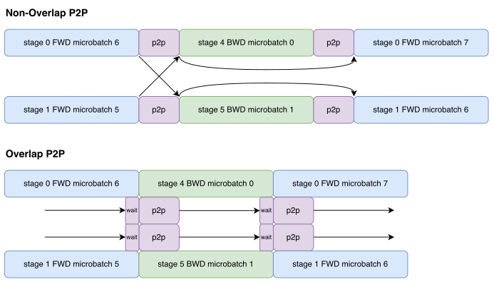
A 1F1B-V handoff cannot be hidden when the receiving rank’s next scheduled action consumes the activation or gradient just produced by its peer. Posting that transfer asynchronously cannot start the dependent kernel earlier: the receiving rank must wait for the tensor at the same schedule step. Other V transfers can still overlap, but hiding this handoff requires changing the schedule and accepting a different bubble or memory trade-off.
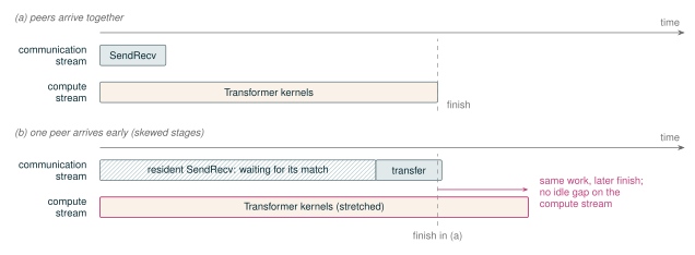
Overlapped P2P still competes for shared resources. The default two-sided NCCL path requires matching send and receive participation. When stage runtimes are skewed, an early peer can leave a resident NCCL send/receive kernel waiting for its match. That kernel can contend with the Transformer kernel intended to hide the transfer, so overlapped compute may run more slowly even when the wait is not visible as an idle gap (Figure 27). Capping the resident kernel’s thread-block count shrinks its footprint but does not remove the rendezvous, and a smaller communication footprint can lengthen the transfer. As in Section 5.9, the net time saved depends on both the exposed wait and the slowdown of concurrent computation.
This contention motivated a one-sided alternative for the pipeline boundary. Prototype NCCL remote memory access (RMA) backends replace the matched send and receive with a producer-side put and a consumer-side wait placed at the latest consume point, so no resident kernel waits for a peer. The prototypes currently work only within a node, while PP boundaries usually span nodes, so the two-sided path remains the default.
Figure 27Interactive · conceptual, no measured quantities
Skew the peers: a waiting SendRecv stretches the compute that hides it
- Resident SendRecv waiting for its match
- SendRecv transfer
- Transformer kernels
- Stretched by the waiting kernel
One rank’s two streams. The peer’s arrival delay, the share of SMs a waiting SendRecv holds, and the transfer times are schematic. The one-sided RMA path is a prototype that works only within a node.
Original report figure
6.4 PP Delays Reuse of Saved EP Payloads
An EP buffer becomes reusable only after its pipeline backward finishes. Section 5.7 introduced the hazard and the lease that guards against it: a dispatched payload saved for Wgrad must not be overwritten before its backward consumer runs. Without PP, a forward’s temporary EP buffers can often be reclaimed by the following backward. PP interleaves several microbatches, so a later forward may arrive while an earlier forward still needs its saved EP payload for weight-gradient computation. Buffer reuse must therefore follow the pipeline schedule and the point at which each saved value’s backward consumer finishes, not simply the order of forward calls. The pipeline schedule determines how many slots must exist at once.
Let \(F_s(t)\) and \(B_s(t)\) count completed forwards and backwards for stage \(s\) by schedule time \(t\). The outstanding-forward high-water \[H_s=\max_t\bigl(F_s(t)-B_s(t)\bigr)\] predicts how many stage-\(s\) payloads can be live concurrently. It sizes a buffer pool, but it does not determine when any particular slot is reusable. A slot becomes reusable only after the matching backward has consumed the saved value.
We encountered this hazard in a PP–EP correctness failure. Rowwise expert execution saved a self-managed symmetric-memory dispatch payload needed later for expert weight gradients. A later pipeline forward could reuse that storage before the matching backward consumed it. The corrupted values could remain finite in BF16, so loss finiteness alone did not rule out a silent wrong gradient; the MXFP8 form of the same bug instead surfaced as an infinite gradient norm from stale scales. The repair uses two complementary rules: the schedule high-water determines how many slots to reserve, while the saved autograd value retains a lease on its particular slot until its backward consumer finishes (Figure 22).
Two schedule features change what the lease rule must cover. Recomputation (Section 13) changes whether a value must survive from the original forward, and two-batch overlap (TBO, Section 15.3) can multiply simultaneous acquisitions within one scheduled forward.
PP peak memory therefore includes not only stage parameters but also the schedule-dependent high-water of ordinary activations, communication buffers, route metadata, and rowwise payload leases. Appendix F describes how context parallelism changes the activation shape entering this same reuse rule.
6.5 Runtime Determines Pipeline Throughput
Once a configuration fits, the microbatch schedule and stage runtimes determine its throughput. Let \(m\) be the number of pipeline microbatches in one optimizer step. Increasing \(m\) amortizes warmup and cooldown because more work occupies the steady-state portion of the pipeline. It does not make those bubbles disappear, and it is not equivalent to increasing the microbatch size. At fixed global batch, increasing \(m\) makes each microbatch smaller, which can reduce attention and GEMM efficiency and increase launch and P2P overhead per token. The useful operating point therefore balances pipeline occupancy against the efficiency of each stage invocation.
One straggling stage throttles the complete pipeline. Equal layer counts are only a starting point because embeddings, the language-model head, dense versus routed blocks, shared experts, recomputation, and routing imbalance all change stage time. In PP recipes where the last virtual stage’s language-model head and loss would make it the straggler, we leave that stage one Transformer block lighter. For example, some nominal 32-block designs use 31 blocks while retaining split points from the 32-block partition, so the missing block comes from the final stage. This is a profile-guided recipe choice, not an automatic scheduler policy. We balance stages using measured time and memory rather than layer count alone.
Symbolic timelines omit execution costs. Generated timelines reveal action order, empty slots, activation high-water, and possible P2P overlap windows. They do not include kernel duration, transfer latency, CPU launch gaps, GPU idle time, or contention between concurrent operations. A smaller symbolic bubble can still lose to smaller microbatch kernels, an imbalanced stage, or communication interference. Pipeline throughput must therefore be measured at runtime for the complete configuration rather than inferred from the schedule diagram alone.
The production operating points in Section 14 report measured throughput for the PP4 and PP8 configurations used at scale.