Section 08: Synchronization-Free Training

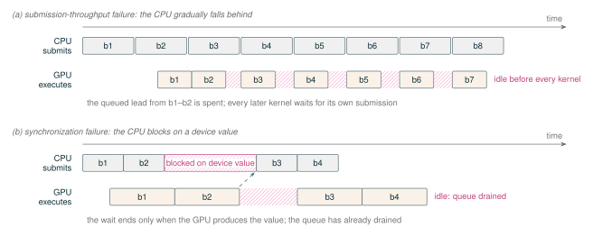
The GPU executes each training step, but the CPU prepares and submits nearly all of that work. A CUDA kernel launch normally returns without waiting for the kernel to finish, allowing the CPU to submit later operations while the GPU executes earlier ones (NVIDIA 2026f; PyTorch Contributors 2026b). This asynchronous execution is essential for high utilization: the GPU should find its next operation already waiting when the current operation finishes. The GPU can run out of queued work if the CPU submits operations too slowly or blocks while waiting for a device-produced value (Figure 29). Slow submission calls for less host work or more device work per launch. A device-to-host wait instead calls for an interface that keeps device results off the host’s steady-state path; initialization, compilation and warmup, and buffer allocation may still synchronize.

Figure 29Interactive · conceptual, no measured quantities · figure time units

Two ways the GPU runs out of queued work

Failure

(a) Slow submission(b) Host waits for a value

Submission period per block (GPU block = 1.00)

1.55report

• CPU submission
• GPU execution
• GPU idle
• Drag, tap or use ← → to move the cursor

CPU at the cursor

submitting b4

GPU at the cursor

idle: waiting for b4’s submission

Queued blocks

0

Per block: one submission every 1.55 vs execute 1.00 (figure units)

If T_submit ≥ T_device, the GPU eventually reaches the end of the submitted queue and waits for the host. Section 8.1

Panel (a) follows the figure’s proportions: a block is submitted every 1.55 figure units, each GPU block takes 1.00, and b1 starts after the lead already queued. The slider re-times the same blocks with one rule: a block starts when its submission is complete and the GPU is free. Panel (b) is drawn as in the report; its numbered steps are the phrases of caption (b).

Figure 29. GPU idle intervals caused by slow submission and host waits. (a) When submitting a block costs the CPU more time than executing it costs the GPU, the queued lead is spent and every later kernel waits for its own submission; the GPU idles a little before every block. (b) When the CPU blocks on a device value, submission stops entirely: the GPU finishes the queued work, sits idle until the value is produced and the host resumes, and the host must then rebuild its lead. Conceptual illustration with no measured quantities.

MoE training is especially sensitive to both problems. Routing introduces many short metadata operations around the expert GEMMs, and the number of tokens assigned to each rank and expert is data dependent. A direct implementation may therefore combine small GPU work units with host-visible counts, variable allocations, and variable communication schedules. These costs are part of the systems tax introduced in Section 1.3; they are not counted by the model-FLOP estimate.

In this section, synchronization-free has a narrow meaning: the steady-state training path contains no avoidable host-blocking synchronization for routing, allocation, communication, or expert scheduling. It does not mean that execution has no ordering. CUDA stream dependencies, collective completion, autograd dependencies, and optimizer-step boundaries are still required. In the MoE path examined here, the all-to-all and grouped GEMM required host-visible counts, which cost one host wait per routed block. Section 8.5 describes how Olmo removes that wait without introducing a new one.

8.1 The CPU Must Stay Ahead of the GPU

Consider a repeated region such as one transformer block. Let \(T_{\mathrm{submit}}\) be the CPU time required to submit the region and \(T_{\mathrm{device}}\) be the time required by its GPU work. If \(T_{\mathrm{submit}} < T_{\mathrm{device}}\), the CPU can usually move ahead while the GPU executes. If \(T_{\mathrm{submit}} \geq T_{\mathrm{device}}\), the GPU eventually reaches the end of the submitted queue and waits for the host. Dependencies and concurrent streams make this comparison a diagnostic, not a complete performance model, but it identifies the relevant imbalance.

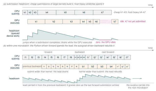
We call the amount of submitted but not-yet-completed GPU work the submission headroom. Headroom is a function of wall-clock time: it jumps up by a kernel’s device duration when the CPU completes that kernel’s submission, drains at unit rate while the GPU executes, and the GPU is idle exactly while it is zero. Large GEMMs, scaled dot-product attention, fused kernels, compiled regions, and C++ execution can build headroom because they submit substantial device work with relatively little host work. Python call stacks, dispatcher and compilation-cache lookups, metadata bookkeeping, and many short launches consume it. Submission headroom is an interpretation of a CPU/GPU timeline, not a CUDA metric: the CPU’s lead over GPU execution shrinks to zero when the device runs out of queued work. Figure 30a draws headroom as this quantity, and Table 12 summarizes which common operations build or consume it. Figure 31 then contrasts a dense block sequence that sustains that lead with a routed one in which a per-block synchronization point removes it.

Backward passes usually rebuild headroom. A layer’s backward launches roughly twice the GPU work of its forward—the input-gradient and weight-gradient GEMMs (Dgrad and Wgrad, Section 9)—while the autograd engine submits that work with less per-launch overhead than the Python-driven forward. The lead earned during one microbatch’s backward then carries into the next microbatch: the first forward blocks can still run with positive headroom, while each submission-bound block spends part of the lead and leaves less for the blocks behind it. Figure 30b shows this drain-and-rebuild cycle within one microbatch.

Figure 30Interactive · conceptual, curves computed from the drawn boxes · figure time units

Scrub the timeline: headroom is the work already waiting on the GPU

Panel

(a) Build and spend(b) One microbatch

Host time per k4–k7 submission (each kernel runs 0.70)

2.00report

• CPU submission (full host cost)
• GPU kernel
• GPU idle
• Headroom H(t)
• Drag, tap or use ← → to step through events

CPU at the cursor

submitting k7 (host-heavy)

GPU at the cursor

idle: k7 not yet submitted

Headroom at the cursor = queued, not-yet-executed device work

0.00 figure units

nothing queued: H = 0

k4–k7: submit 2.00 vs execute 0.70

after the lead reaches zero the GPU waits for k7’s submission caption (a)

The curve applies the caption’s rule to the report’s boxes. The slider changes one submission cost and re-runs the same rule (a kernel starts when it is submitted and the GPU is free); the report’s value is marked.

Figure 30. Submission headroom is the queued, not-yet-executed device work. Both curves are computed exactly from the drawn boxes: headroom jumps up by a kernel’s device duration when the CPU completes that kernel’s submission and drains at unit rate while the GPU executes, so the GPU is idle exactly where the curve sits at zero. (a) Cheap submissions of large kernels (k1–k3) build the lead; a host-heavy stretch of small kernels (k4–k7) spends it faster than it is replaced, and after the lead reaches zero the GPU waits for k7’s submission. (b) Within one microbatch, each Python-driven forward submission costs the CPU more time than its kernel costs the GPU, so the lead carried in from the previous backward drains layer by layer and grazes zero just as the last forward submission arrives. The autograd-driven backward inverts the imbalance, and while the GPU executes it, the CPU is already submitting the next microbatch’s forward: the rebuilt surplus is the lead that forward will spend. Each CPU box’s width is the full host cost of its submission, including Python and dispatcher time. Conceptual illustration with no measured quantities.

The distance between an API launch on the CPU and the corresponding GPU start is useful, but it must be interpreted with stream dependencies. A long distance can mean that useful work is already queued, or that the operation is waiting on another stream. The decisive observation is whether the GPU has runnable work when the preceding operation completes. GPU utilization and power are too coarse to establish this cause by themselves.

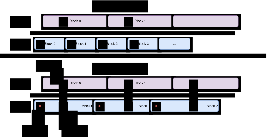
Figure 31Interactive · conceptual, order only · no measured duration

Scrub both timelines: how far ahead can the CPU get?

• CPU submits a block
• GPU executes it
• Sync wait (red dot: start; black dot: end, at the GPU’s sync point)
• Blocks ahead, dense
• Blocks ahead, MoE
• Drag, tap or use ← → to step

Dense model

CPU on a later block · GPU on Block 1

CPU ahead by 3 blocks

MoE model

CPU waits at Block 2’s sync point until the GPU reaches it

CPU ahead by 1 block

Why it matters

Submission headroom cannot accumulate beyond one block, so the two processors advance in lock step and any GPU stall is exposed. Figure caption

Boxes and dots are placed as in the report figure. “Blocks ahead” counts how many blocks the CPU’s current block is ahead of the GPU’s: the dense CPU runs several blocks ahead (three in the drawn span, counting the “…” block), the MoE CPU never more than one.

Figure 31. A per-block synchronization point stops the CPU from running ahead. In the dense timeline (top), the CPU submits blocks well in advance of their GPU start times, so several blocks of device work stay queued and the GPU always finds its next operation waiting. In the routed timeline (bottom), every block contains a synchronization point: the CPU begins a sync wait, blocks until the GPU reaches the matching point, and only then submits the remainder of the block. Submission headroom cannot accumulate beyond one block, so the two processors advance in lock step and any GPU stall is exposed. The timeline is conceptual and does not encode measured duration. Section 8.4 examines the synchronizing operations themselves.

Captured profiles of the eight-layer development model show both timeline shapes, one per expert-parallel path (Figure 74 in Appendix B.5). In the synchronized trace, a host wait inside every routed block keeps the CPU and GPU spans of each forward block aligned, and the kernel rows show idle gaps at the block boundaries. In the rowwise trace, the CPU submits an entire microbatch while the GPU is still executing earlier work, and the GPU then executes the submitted blocks back to back.

8.2 Small Work Units Expose Submission Overhead

For a fixed operator sequence, a simple host-time approximation is

\[ T_{\mathrm{submit}} \approx N_{\mathrm{launch}}\,t_{\mathrm{launch}} + T_{\mathrm{framework}} + T_{\mathrm{bookkeeping}}, \tag{11} \]

whereas the GPU time of its GEMMs and attention generally grows with the number of tokens. Reducing the microbatch can therefore shorten device execution without reducing host work in proportion. This is one reason that a kernel-level speedup may disappear when the same kernels are invoked through an eager training stack.

Routed blocks add host submission work to the transformer operations shared with a dense model: each block constructs routing metadata, counts expert assignments, attaches router losses, permutes or maps rows, launches expert communication, and schedules grouped GEMMs. Expert parallelism can also divide the local tokens among many experts, making each GEMM shorter. The resulting sequence of short GPU operations leaves less time for the CPU to prepare the next group of launches, even when each operation is cheap in isolation.

The same reasoning applies to very fast normalization, elementwise, and reduction kernels. Their device time can be shorter than the framework and launch path around them. The appropriate remedies are then larger work units, fusion, compilation, or a lower-overhead C++ interface. These remedies reduce ordinary submission cost; they do not remove an explicit device-to-host wait. The balance between submission and execution sets the microbatch-size crossover discussed next.

8.3 Critical Microbatch Size

This host–device balance defines a systems critical microbatch size. It is unrelated to the optimization-theoretic critical batch size discussed in Section 16. Let \(b\) denote the rank-local amount of work in one microbatch—for example, the number of sequences at fixed sequence length—and compare the CPU submission time \(T_{\mathrm{submit}}(b)\) with the corresponding GPU execution time \(T_{\mathrm{device}}(b)\). The crossover occurs near

\[ T_{\mathrm{device}}(b_{\mathrm{crit}}) \approx T_{\mathrm{submit}}(b_{\mathrm{crit}}). \tag{12} \]

Below this point, the GPU completes the submitted work faster than the CPU can prepare and launch the next work, so the GPU can run out of queued operations and become idle. At or above the crossover, each submitted region contains enough device work for the CPU to stay ahead. This threshold is not a model constant: it depends on the operator mix, fusion and compilation boundaries, software stack, CPU, GPU, and sequence length.

The crossover must be identified from the CPU/GPU profile of the selected configuration. Figure 32 illustrates how it can move; it does not estimate a critical size for a production run.

Figure 32Interactive · conceptual, qualitative schematic · no measured values

Move the microbatch: where does each GPU stop running dry?

GPU

H100B200B300

CPU submission

EagerReduced overhead e.g. CUDA Graph

Each marked crossover is where device time meets submission time, the condition of Equation 12. Curves are the schematic functions of the report’s plotting script (H100, B200 and B300 execution time; CPU submission time, eager and with CUDA Graph replay as one way to reduce overhead), in the script’s colours. The H100 and B200 curve ends mark the drawn VRAM limits.

Figure 32. A faster GPU can move the critical microbatch size to the right. The solid red curve represents CPU submission time, while the blue, purple, and green curves represent H100, B200, and B300 execution time. Below a crossover, the device can consume work faster than the host supplies it; faster execution with an unchanged host path therefore requires a larger microbatch to restore submission headroom. Additional GPU memory can extend the feasible microbatch range, while reducing submission overhead (dashed red; CUDA Graph replay is one way to reduce this overhead) can move the crossover to the left. The curves, intersections, and memory limits are qualitative annotations rather than measurements; no numerical critical size is implied.

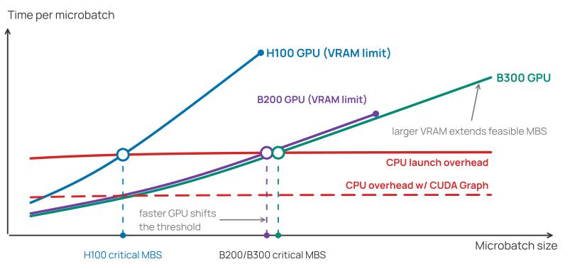
This trend matters as accelerators improve. Moving from Hopper to Blackwell can shorten the device side of the same operator sequence without reducing Python, dispatcher, routing-bookkeeping, or launch work by the same factor. The crossover can therefore shift to a larger microbatch. A configuration that kept an H100 continuously supplied may become host-submission limited on a faster GPU even though every individual GPU kernel improved.

Memory-saving techniques can keep the GPU supplied by making a larger microbatch feasible: lower-precision activation storage and activation recomputation reduce the per-token memory cost, as discussed in Sections 11 and 13. Cheaper submission instead moves \(b_{\mathrm{crit}}\) to the left: fusion, compiled regions, and C++ execution reduce repeated host work in the production path, and CUDA Graph replay provides a low-host-overhead reference (NVIDIA 2026g; PyTorch Contributors 2026b). Larger microbatches consume more activation memory, while static PyTorch capture/replay imposes address, shape, and buffer-retention constraints; their value depends on whether CPU submission or GPU execution limits the measured step at the selected microbatch size.

8.4 Device-to-Host Synchronization Drains the Queue

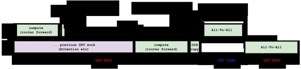
A device-to-host (D2H) synchronization occurs when host execution cannot continue until a value computed on the GPU is available to the CPU. The CPU stops submitting later work while the GPU completes all dependencies needed to produce that value. The wait consumes submission headroom, but the GPU becomes idle only if it outlasts useful independent work that was already submitted. After the value arrives, the host must rebuild its lead over the device.

Block all-to-all EP (Section 5.3) provides a concrete example. Routing produces the number of tokens sent to each destination on the GPU. In Olmo-core’s synchronized path, ranks exchange token counts on the GPU, then copy the send, receive, and local-expert counts to CPU memory and wait. The send and receive counts become the Python split lists used to launch the data exchange. A fully dynamic receive buffer has the same problem when its allocation shape is derived from device counts. Some legacy grouped-GEMM backends¹ likewise require host-visible expert sizes, although that dependency can occur without EP. The simplified pseudocode shows one host copy and wait serving both host dependencies:

peer_sizes_gpu = count_routes_per_peer(routes)
expert_sizes_gpu = count_routes_per_expert(routes)
peer_sizes, expert_sizes = copy_to_cpu_and_wait( # host sync
    peer_sizes_gpu, expert_sizes_gpu)
# All-to-all requires host-side split sizes.
all_to_all(x, split_sizes=peer_sizes)
# Legacy grouped GEMM also requires host-side expert sizes.
grouped_gemm(x, expert_sizes)

Both dependencies arise when an interface turns device-produced counts into host inputs. A receive buffer allocated from the current route count creates the same dependency even if the transfer itself accepts device metadata. Section 8.5 follows the changes to communication, allocation, and grouped-GEMM scheduling that keep these counts on the GPU.

Figure 33Interactive · conceptual, order only · no measured duration

Where the all-to-all waits: follow the route counts

Count consumer

Host split sizes as in the report figureDevice route map web sketch of §8.5

• CPU launch
• GPU work
• CPU waits
• GPU idle
• Drag, tap or use ← → to step through events

CPU at the cursor

submitting All-To-All

GPU at the cursor

idle: nothing runnable is queued

All-to-all

launched only after the counts are host-visible

If the queue drains at this boundary, the GPU becomes idle until the host receives the counts and submits the all-to-all. Figure caption

Boxes are placed as in the report figure (draw.io geometry). The “device route map” view is a conceptual sketch of the rowwise path in Section 8.5, not a report figure: counts, offsets and the dispatch input stay CUDA tensors, and the count exchange stays on the GPU. Required device ordering remains in both views.

Figure 33. Host-visible split sizes delay the all-to-all launch. The GPU produces route counts, but the synchronized variable-split path must expose them to the CPU before the collective can be launched. If the queue drains at this boundary, the GPU becomes idle until the host receives the counts and submits the all-to-all. The timeline is conceptual and does not encode measured duration.

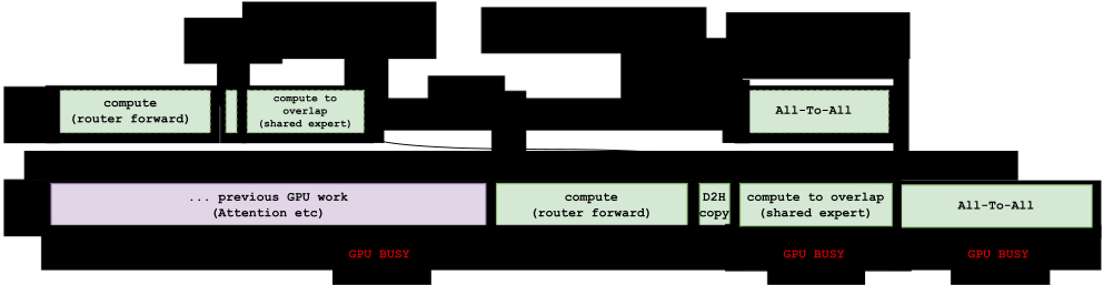
Independent work submitted before the host wait can occupy some or all of this interval. In Figure 34, shared-expert compute runs while the CPU waits for the route counts. This scheduling hides the GPU bubble but does not remove the synchronization or allow the all-to-all to launch before its split sizes reach the host.

Figure 34Interactive · conceptual, order only · no measured duration

Cover the wait, not remove it: slide independent work into the bubble

Independent work submitted before the wait (shared expert)

as drawnreport

• CPU launch
• GPU work
• CPU waits
• GPU idle
• Drag, tap or use ← → to step through events

CPU at the cursor

submitting All-To-All

GPU at the cursor

executing compute to overlap (shared expert)

All-to-all

launched only after the counts are host-visible

Covered, as drawn in the report: the GPU remains busy while the host waits Figure caption

This scheduling hides the GPU bubble but does not remove the synchronization or allow the all-to-all to launch before its split sizes reach the host. Section 8.4

Slide to zero to recover Figure 33; the report figure’s shared-expert work is marked. Above zero only the GPU lane changes; at zero the CPU lane returns to Figure 33’s (no shared-expert launch before the wait). Gaps narrower than the report’s own gaps between boxes count as busy, as in the report’s GPU BUSY bar.

Figure 34. Independent compute can cover a host wait without removing it. The CPU submits shared-expert work before blocking on GPU-produced route counts, so the GPU remains busy while the host waits. The all-to-all still cannot be submitted until the counts are host-visible. This is latency coverage, not communication–compute overlap; the timeline is conceptual and does not encode measured duration.

Dynamic routing itself does not require a host synchronization. The synchronization is introduced by an interface that asks the CPU to interpret a device result. Table 13 separates definite host-visible operations from operations that are often blamed incorrectly.

PyTorch explicitly documents the synchronization behavior of nonzero() on CUDA (PyTorch Contributors 2026k). Scalar extraction and host-visible copies have the same fundamental dependency: Python cannot use a value that the device has not produced. This does not imply that every dynamic operator or tensor allocation synchronizes. Whether a hot-path call blocks depends on where its shape and control data reside.

CUDA stream events illustrate the distinction between required device ordering and host blocking. A stream can wait on an event while the CPU continues to submit independent work. Calling a host synchronization routine waits on the CPU and therefore changes the submission path. The goal is to retain necessary device ordering without making the host participate in data-dependent scheduling.

8.5 How to Become Synchronization-Free

Device-resident route metadata and device-side grouped-GEMM offsets remove the host-visible counts that the all-to-all and grouped GEMM required, and with them the per-block host wait, from Olmo’s rowwise MoE path. Capacity-shaped storage prevents route counts from becoming host allocation decisions. The selected routes remain dynamic; buffer capacities are fixed before the training loop.

The rowwise mechanics are those of Sections 5.4 and 5.7; this subsection isolates their host-facing consequence. Table 14 lists the host dependency removed by each mechanism and its associated cost. The first two rows remove the all-to-all dependency; the third removes the grouped-GEMM dependency. Each removal has a focused illustration: Figures 15 and 16 contrast the synchronized block all-to-all with the rowwise path whose route metadata never leaves the GPU, and Figures 36 and 37 contrast the host-loop grouped GEMM with the device-scheduled interface that consumes offsets where they are produced.

Device-resident route metadata.

The router produces route maps, destination ranks and rows, per-rank counts, and expert-group offsets as CUDA tensors. The rowwise dispatch and combine kernels consume those tensors directly (Figure 16). Olmo currently uses NVSHMEM because it supports GPU-initiated one-sided PUT and GET operations over symmetric memory (NVIDIA 2026s). The host still launches kernels and establishes the communication resources; it does not retrieve a variable split list for each microbatch. Per-rank count exchange, stream waits, and NVSHMEM barriers still provide required device ordering; their route-dependent values remain CUDA tensors and are not consumed by the host. The count exchange is one all-gather over the EP-MP group. This is the rowwise NVSHMEM path analyzed in this section.

Capacity-shaped storage.

Dispatch, combine, scale, and metadata buffers are allocated to a configured capacity. A route map identifies which rows are valid in the current microbatch. This separates a static upper bound, which the allocator needs, from the dynamic valid-row count, which remains on the device. The distinction matters because unwritten capacity rows may contain stale data; expert compute and combine therefore consume only the rows marked valid for the current microbatch.

Device-side grouped-GEMM scheduling.

Current Olmo expert compute uses a grouped-GEMM interface with a CUDA int32 cumulative-offset tensor (Figure 37). The backend, rather than a Python loop, identifies the row range assigned to each local expert. This removes the need to call item() on each expert count and also reduces the number of GEMM launches. A CPU-loop implementation would instead copy offsets to the host and serialize group launches, recreating the synchronization and launch gaps that the device-offset interface removes.

Capacity trades memory for the removed stall.

A fixed envelope can reserve more memory than the valid routes require and can drop routes if the configured capacity is exceeded. Current grouped GEMMs use device offsets and stop at the valid expert rows (Section 9), but capacity tails still occupy buffer memory and can be touched by non-GEMM elementwise work; a tail-aware SwiGLU kernel that applies the activation only to the valid prefix avoids touching the tails on forward-only paths. Other implementations may also communicate padded rows. Useful-token FLOPs must exclude those rows, while physical memory, transferred bytes, and executed kernel work must include them. Capacity overhead is therefore the cost of removing the host synchronization.

Reducing remaining submission overhead.

Fusion, compiled regions, and C++ execution reduce the number and cost of ordinary launches after dynamic metadata has been kept on the device. These techniques solve a different problem from D2H synchronization. A faster Python or C++ call stack cannot repair an API that fundamentally requires a GPU value in Python. In the current implementation, the custom symmetric-memory transport remains a deliberate C++/CUDA boundary of the compiled block; compilation reduces surrounding work but does not capture the complete rowwise path as one graph.

CUDA Graph replay could remove much of this remaining submission cost, but its stable-address and fixed-shape requirements conflict with live pipeline microbatches, and the production path is not graph captured. Section 15.6 analyzes that trade and uses replay only as a diagnostic ceiling that separates device service time from eager submission cost.

Host-wait behavior depends on the running configuration. Appendix B.6 records the verification checklist and a graph-replay microbenchmark that isolates the submission tax on short expert operations. In the captured rowwise timeline of Appendix B.5, no host wait interrupts submission for the eight-layer BF16 EP8 development model with a shared expert. This is a single-rank captured instance of the mechanism, not a guarantee for every configuration or execution phase; initialization, compilation, warmup, and buffer allocation remain outside the steady-state scope.

Capacity memory and padding remain costs of this design. Once the count-dependent wait is removed, ordinary submission overhead still determines whether the CPU can keep the GPU supplied.