
A routing decision is both a model choice and a distributed-work request. For each token, the router produces soft scores and selects \(K\) experts, creating \(K\) requested routes. Capacity then determines which requests are kept. Dispatch moves the kept rows to the expert-owning ranks; on the rowwise real-count path, grouped GEMM executes their densely packed expert segments, and combine returns their weighted contributions. Requested and kept routes coincide when no route is dropped, but they are different objects whenever capacity overflows.
Load-balancing mechanisms influence future requests, while capacity limits how many of the current requests are admitted. The resulting workload has both an expert-level shape and a destination-rank total. The former controls expert training signal and grouped GEMM geometry, while the latter controls communication, buffer use, overflow, and straggling. After establishing those systems consequences, we compare the scopes and mechanisms used to balance routes and then analyze a failure of the standard Switch-style auxiliary objective (Fedus et al. 2022): its scalar can fall while requested routing becomes less balanced.
Requested Routes and Kept Routes
The current load-balancing loss (LBL) and post-batch bias controller (Section 10.6) use requested top-\(K\) assignments. Capacity and dispatch use kept assignments, and the rowwise path also uses their real counts for grouped GEMM. When routes are dropped, neither histogram is a substitute for the other.
10.1 From Top-\(K\) Selection to the Executed Workload
Consider one routed layer with \(N\) global experts and \(M_E\) expert-parallel ranks. Let source rank \(s\) hold \(T_s\) tokens, and let \(S_{s,t}\) be the \(K\) experts selected for token \(t\). One pair \((t,i)\) with \(i\in S_{s,t}\) is a route. The number of routes requested from source rank \(s\) to expert \(i\) is \[ C_{s,i}^{\mathrm{req}} \mathrel{:\mkern-0.25mu=}\sum_{t=1}^{T_s}\mathbf{1}\{i\in S_{s,t}\}, \qquad \sum_{i=1}^{N}C_{s,i}^{\mathrm{req}}=KT_s. \tag{19} \] Aggregate over sources to obtain the global requested count \(C_i^{\mathrm{req}}\mathrel{:\mkern-0.25mu=}\sum_s C_{s,i}^{\mathrm{req}}\). If \(\rho(i)\) is the expert-parallel rank that owns expert \(i\), the total demand placed on destination rank \(q\) is \[ R_q^{\mathrm{req}} \mathrel{:\mkern-0.25mu=} \sum_{i:\rho(i)=q}C_i^{\mathrm{req}}. \tag{20} \] Thus the same top-\(K\) decisions define two workload distributions: counts over experts and sums over the experts colocated on each destination rank.
Capacity acts between requested routes and execution. Let \(C_{s,i}^{\mathrm{keep}}\) be the routes admitted by the capacity policy and define \[ \begin{aligned} D_{s,i} &\mathrel{:\mkern-0.25mu=}C_{s,i}^{\mathrm{req}}-C_{s,i}^{\mathrm{keep}}, & C_i^{\mathrm{keep}} &\mathrel{:\mkern-0.25mu=}\sum_s C_{s,i}^{\mathrm{keep}},\\ D_i &\mathrel{:\mkern-0.25mu=}C_i^{\mathrm{req}}-C_i^{\mathrm{keep}}, & M_i &\mathrel{:\mkern-0.25mu=}C_i^{\mathrm{keep}}, & R_q^{\mathrm{keep}} &\mathrel{:\mkern-0.25mu=}\sum_{i:\rho(i)=q}C_i^{\mathrm{keep}}. \end{aligned} \tag{21} \] Here \(D_{s,i}\) and \(D_i\) count source-specific and aggregate dropped routes, \(M_i\) is the row count actually presented to expert \(i\) (the per-expert row count of Section 9; its subscript is an expert index, not the rank count \(M_E\)), and \(R_q^{\mathrm{keep}}\) is the actual receive and compute load on rank \(q\). Write \(\boldsymbol{C}^{x}=(C_1^x,\ldots,C_N^x)\) for \(x\in\{\mathrm{req},\mathrm{keep}\}\). In a no-drop step, \(C_{s,i}^{\mathrm{keep}}=C_{s,i}^{\mathrm{req}}\); otherwise the distinction is essential. A kept histogram can appear benign only because excess demand was dropped, while a requested histogram alone does not describe the work that ran. Table 16 records which part of the training system produces and consumes each routing quantity.
| Quantity | Created by | Consumed by |
|---|---|---|
| Router score or logit | Router projection and gating function | The configured score or logit drives top-\(K\); selected unbiased affinities or logits determine mixture weights; normalized all-expert scores form LBL’s differentiable term |
| Requested count \(C^{\mathrm{req}}\) | Top-\(K\) expert identifiers | LBL’s detached hard term, post-batch bias feedback, and capacity admission; on the rowwise path, all-gathered requested splits form the keep matrix that determines dispatch destination ranks and row offsets |
| Kept count \(C^{\mathrm{keep}}\) | Capacity keep/drop policy | Dispatch and combine payload; expert grouped GEMM row counts on real-count paths; and executed-work diagnostics |
Olmo uses token-choice routing: every token selects experts (Shazeer et al. 2017). BASE Layers instead solves a balanced assignment, and Expert Choice lets each expert select tokens; these alternatives change which side of the token–expert relation imposes the constraint (Lewis et al. 2021; Zhou et al. 2022). The remainder of this section concerns Olmo’s token-choice path.
10.2 The Costs of Imbalance Depend on Where It Appears
For any nonzero load vector \(\boldsymbol{x}\in\mathbb{R}_{\geq0}^{n}\) with \(n>1\), define its max/mean imbalance as \[ I_{\max}(\boldsymbol{x}) \mathrel{:\mkern-0.25mu=} \frac{\max_j x_j}{\frac{1}{n}\sum_jx_j} = n\frac{\lVert\boldsymbol{x}\rVert_\infty} {\lVert\boldsymbol{x}\rVert_1}. \tag{22} \] Applying this definition to requested expert counts, kept expert counts, requested destination-rank totals, and kept destination-rank totals answers four different questions (Table 17). The expert-level pair describes selection and executed expert shapes; the rank-level pair describes demand and admitted work at the rank that can become a straggler.
| Counts | Over experts | Over destination ranks |
|---|---|---|
| Requested | Selection concentration: the training signal the router asks for | Demand on the hottest rank: capacity pressure and drop risk |
| Kept | Executed expert shapes presented to grouped GEMM | Admitted receive, compute, and combine load on the rank that can straggle |
Max/mean identifies the hottest coordinate but does not describe how the remaining load is distributed. Let \(\pi_j=x_j/\sum_\ell x_\ell\) be the normalized load distribution and \(H(\boldsymbol{\pi})=-\sum_j\pi_j\log\pi_j\) its entropy. The number of never-selected experts, coefficient of variation, and normalized entropy deficit \(I_H(\boldsymbol{x})=1-H(\boldsymbol{\pi})/\log n\) capture complementary aspects of concentration. The source–destination request matrix contains more communication information than its row or column sums: it resolves which source rank sends how many rows to which destination rank, the per-pair traffic that row and column totals average away. Drop rate and receiving-buffer utilization then show how capacity transformed demand into executed work.
The model-side selection pattern starts with requested expert counts, but routed-expert activations and gradients follow kept counts. An expert can be requested yet receive no signal from a dropped route. At the other extreme, requiring every small or domain-homogeneous microbatch to be uniform can oppose useful specialization. The desirable distribution is therefore scope-dependent: avoiding starvation over the training population does not require every local microbatch to look uniform (Qiu et al. 2025).
The systems-side effect starts with kept counts. Even at a fixed rank total, concentrating rows into fewer experts changes the shapes presented to grouped GEMM. Section 9 measured this directly: as the expert-load histogram concentrated, normalized grouped-GEMM throughput declined with entropy deficit, and median throughput in the most-concentrated entropy range ran about seven points below the least concentrated (Figure 40). A matched appendix comparison further shows that a single-spike and a three-hot-expert histogram with the same maximum load can have different grouped-GEMM times (Figure 72). These fixed-work microbenchmarks isolate local expert computation; they do not include dispatch, cross-rank waiting, or a learned-router trajectory.
Destination-rank imbalance adds those omitted costs. A rank with high \(R_q^{\mathrm{req}}\) consumes capacity faster and is more likely to drop routes. A rank with high \(R_q^{\mathrm{keep}}\) receives more rows, performs more expert work, returns more outputs, and can delay peers or a pipeline stage. Expert-level and rank-level imbalance can also move independently: a rank may receive a balanced total that is concentrated in one of its local experts, or several moderately hot local experts may make the whole rank a straggler, so diagnostics need both levels.
10.3 Rank-Wide Capacity Bounds Work Without Balancing It
Let \(T_{\mathrm{route}}=KT_s\) be the number of routes produced by one source expert-parallel rank. When source ranks hold equal token counts and each destination owns the same number of experts, balanced expert routing places an average of \(T_{\mathrm{route}}\) requested rows on each destination rank: the factor \(M_E\) from all sources cancels the probability \(1/M_E\) of choosing any one destination. Olmo’s rowwise sync-free path reserves the destination-rank budget \[ C_{\mathrm{rank}} \mathrel{:\mkern-0.25mu=} \max\!\left(1,\left\lceil c\,T_{\mathrm{route}}\right\rceil\right), \tag{23} \] where \(c\) is the capacity factor. This is one shared limit for all experts owned by the destination rank, not one independent limit per local expert. If the rank owns \(N_{\mathrm{local}}\) experts, its balanced per-expert mean is \(T_{\mathrm{route}}/N_{\mathrm{local}}\). The rank budget alone can therefore fit one expert at approximately \[ \frac{C_{\mathrm{rank}}} {T_{\mathrm{route}}/N_{\mathrm{local}}} \approx cN_{\mathrm{local}}, \tag{24} \] times that mean if its neighbors are sufficiently cool. This is a bound on what can fit, not evidence that a trained router reaches it.
The shared budget lets a hot local expert use capacity left unused by cooler local experts while the aggregate admitted demand remains within \(C_{\mathrm{rank}}\). A conventional independent expert capacity instead assigns each of the \(N_{\mathrm{local}}\) experts a limit near \[ C_{\mathrm{expert}} \approx \left\lceil \frac{c\,T_{\mathrm{route}}}{N_{\mathrm{local}}} \right\rceil. \tag{25} \] At approximately the same aggregate reserved rows, that policy can drop routes to one hot expert while neighboring experts leave their allocations unused (Lepikhin et al. 2021; Fedus et al. 2022). The rank-wide rule trades an individual expert bound for flexible sharing within a destination-rank bound.
Reserved capacity and executed rows are also distinct. Olmo’s rowwise NVSHMEM path allocates capacity-shaped receive and combine buffers but packs valid rows densely at the front. If the kept local-expert counts are \((M_1,\ldots,M_{N_{\mathrm{local}}})\), the grouped-GEMM offsets are \[ o_j\mathrel{:\mkern-0.25mu=}\sum_{i=1}^{j}M_i, \qquad j=1,\ldots,N_{\mathrm{local}}. \tag{26} \] Only \([0,o_{N_{\mathrm{local}}})\) belongs to expert compute. Unused capacity rows lie outside every expert interval and may contain stale values. On this path, communication uses fixed capacity but grouped GEMM processes no padding rows: the device-side real-count offsets described in Sections 8 and 9 separate physical allocation from logical work. Other dispatch paths may instead pass capacity-padded splits to expert compute.
On every capacity-enabled sync-free forward, all expert-parallel ranks all-gather their requested split counts and independently derive the same deterministic keep matrix. For each destination, the current policy flattens counts in local-expert-major, then source-rank order, cumulatively admits routes until it reaches \(C_{\mathrm{rank}}\), and keeps a prefix within each source/expert split. Restoration and combine mask the tail-dropped routes. This makes overflow bounded and reproducible, but the ordering can affect which routes survive; a capacity evaluation should therefore report the distribution of drops, not only their total.
The aggregate route-drop fraction is \[ \delta_{\mathrm{route}} \mathrel{:\mkern-0.25mu=} \frac{\sum_{s,i}D_{s,i}} {\sum_{s,i}C_{s,i}^{\mathrm{req}}} = \frac{\sum_{s,i}D_{s,i}}{\sum_sKT_s}. \tag{27} \] For \(K>1\), this is not the fraction of tokens that lose every routed contribution. A model-quality analysis should separately report tokens that lose at least one route, tokens that lose all \(K\), and the selected mixture weight removed by dropping.
Capacity Bounds Admitted Work
Capacity bounds the receive-buffer storage and the worst-case admitted rank work after an outlying routing event. It filters requests after selection; the bound itself provides no guarantee of balanced requested load. The intended regime is nearly dropless under the observed routing distribution: balancing keeps normal demand within the fixed budget, while capacity handles rare excursions. This is not an unconditional dropless guarantee.
10.4 A Shared Rank Budget Drops No More Routes than Matched Expert Budgets
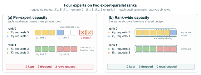
Two capacity policies can reserve the same aggregate rows on a destination rank yet admit different subsets of a skewed request histogram. Figure 41 shows the mechanism on one four-expert example, and Table 18 compares the two allocation policies.
Figure 41Interactive · conceptual, no measured quantities
Private rows for each expert, or one shared budget per rank
Destination rank 0
Destination rank 1
(a) Per-expert capacity
each local expert owns 3 private rows
10 kept2 dropped2 rows unused
(b) Rank-wide capacity
the same 6 rows form one shared budget
12 kept0 dropped0 rows unused
kept routereserved row, unusedunused while a local neighbor overflowsdropped routeadmitted only by sharingtail-dropped, though a private limit would keep it
Point at, tap, or tab to a block to read what happens to that route or row. Use − and + to change a request.
Total drops · Equation 28
| Rank | Rank-wide Drank = [Σj Creqj − B]+ | Per-expert Dexpert = Σj [Creqj − bj]+ |
|---|---|---|
| Rank 0 | [5 + 1 − 6]+ = 0 | [5 − 3]+ + [1 − 3]+ = 2 |
| Rank 1 | [3 + 3 − 6]+ = 0 | [3 − 3]+ + [3 − 3]+ = 0 |
| Both ranks | 0 | 2 |
Dominance · Equation 29
Drank = 0 < 2 = Dexpert
“The inequality is strict when a hot expert exceeds its private budget while a neighbor leaves rows unused.” (Section 10.4)
“Report example” is the original figure’s input (E0: 5 and E1: 1 on rank 0; E2: 3 and E3: 3 on rank 1; 6 rows per rank). Other inputs are illustrative. Per-expert limits are half the rank budget (b = B/2), so both policies reserve the same aggregate rows. Rank-wide admission takes local experts in order (E0 before E1), as the current policy flattens counts in local-expert-major order; kept rows are packed at the front of the buffer, and o1, o2 mark the grouped-GEMM offsets of Equation 26.
Original report figure
| Policy | Allocation unit | Unused capacity and overflow | Expert compute |
|---|---|---|---|
| Independent per expert | One limit for each local expert | Rows reserved by a cool expert cannot admit routes for a hot neighbor; overflow is expert-local | Padded BMM may execute capacity rows; grouped GEMM can still use real kept counts |
| Shared rank-wide | One aggregate limit for the destination rank | Local experts draw from one budget; overflow begins only when their aggregate fills the rank budget | Olmo’s rowwise path packs kept rows and uses real cumulative offsets; another sync-free path can execute capacity-padded splits |
At exactly matched aggregate rows, the drop advantage from pooling unused capacity is algebraic. Given a destination-rank total budget \(B\) and independent expert budgets \(b_j\) satisfying \(\sum_jb_j=B\), the total drops for requested local-expert counts \(C_j^{\mathrm{req}}\) are \[ \begin{aligned} D^{\mathrm{rank}} &= \left[\sum_jC_j^{\mathrm{req}}-B\right]_+,\\ D^{\mathrm{expert}} &= \sum_j\left[C_j^{\mathrm{req}}-b_j\right]_+, \end{aligned} \qquad [z]_+\mathrel{:\mkern-0.25mu=}\max(z,0). \tag{28} \] Because \([\sum_jz_j]_+\leq\sum_j[z_j]_+\), \[ D^{\mathrm{rank}}\leq D^{\mathrm{expert}}. \tag{29} \] A shared rank budget therefore cannot drop more routes in total than independent expert budgets with the same aggregate rows. The budgets must match after integer rounding; a shared nominal capacity factor alone need not give equal aggregate rows. The inequality is strict when a hot expert exceeds its private budget while a neighbor leaves rows unused. It does not prove a universally better training policy: rank-wide tail-drop may preserve a different set of tokens and deliberately gives up the stronger per-expert workload bound.
Per-expert capacity is the standard drop-and-pad formulation in GShard and Switch Transformer (Lepikhin et al. 2021; Fedus et al. 2022). Megatron-Core likewise documents both a per-expert capacity factor and, for the HybridEP and NCCL-EP backends of its flex token dispatcher, a per-expert-rank capacity factor (NVIDIA 2026k). Comparisons therefore need to specify the capacity policy for the backend and revision being compared.
Capacity reacts to overload after selection. Balancing instead changes future requested demand, beginning with the token scope over which that demand is measured.
10.5 Load-Balancing Scope Is Part of the Training Objective
The balance batch is the set of tokens used to construct the requested hard frequency vector. It need not coincide with the optimizer batch, and changing it changes the training objective even when the language-modeling batch, optimizer, and model are unchanged. A narrow scope asks every small token group to use the experts uniformly; a broad scope allows imbalance within one sequence, rank, domain, or microbatch as long as it is compensated elsewhere in the balance batch. The latter can reduce conflict between load balancing and specialization when microbatches are small or domain-homogeneous (Qiu et al. 2025).
For a balance batch of \(T\) tokens, \(N\) routed experts, and \(K\) selections per token, let \(f_i=C_i^{\mathrm{req}}/(KT)\) be expert \(i\)’s fraction of requested routes before capacity, and let \(P_i=T^{-1}\sum_{t=1}^{T}p_{t,i}\) be its mean router score, with \(p_{t,i}\) normalized across experts for each token. The Switch-style load-balancing loss couples these two statistics (Lepikhin et al. 2021; Fedus et al. 2022): \[ \mathcal{L}_{\mathrm{LBL}} \mathrel{:\mkern-0.25mu=}N\sum_{i=1}^{N}f_iP_i = N\boldsymbol{f}^{\mathsf T}\boldsymbol{P}. \tag{30} \] The hard fractions \(f_i\) are treated as constants; gradients flow through \(P_i\). The factor \(N\) keeps the balanced value equal to one as the expert count changes. The external coefficient multiplying this loss in the training objective is omitted here.
Table 19 separates five relevant scopes, including three distributed or accumulation-aware variants that are often conflated under “global load balancing.” Only the first two are implemented as Olmo LBL granularities today.
| Scope | Statistics and semantics | Coordination and cost | Olmo status |
|---|---|---|---|
| Instance | One per-sequence hard histogram, reduced across tensor- and context-parallel shards as applicable, paired with each shard’s local differentiable soft-score contribution | Reductions induced by sequence sharding | Implemented as instance |
| Rank-local microbatch | Current rank’s current microbatch; unrelated local sequences can compensate, while CP shards remain local | No additional count communication | Implemented as local_batch |
| Synchronized current microbatch | Current hard counts reduced over the stage-local token balance group; each rank contributes its local soft term | One \(N\)-element count all-reduce per routed-layer forward | Design only |
| GA-buffered online global | Synchronized counts accumulated through gradient accumulation; microbatch \(m\) uses the prefix through \(m\) | Same all-reduce plus an \(N\)-element per-router buffer | Design only; analogous to Megatron global_aux_loss |
| Exact optimizer-batch global | Final hard counts and soft-score sums over all ranks and all accumulation microbatches | Delayed backward, retained graphs, or a routing prepass; stale statistics instead define an approximation | Not implemented |
The last two rows are not interchangeable. Let \(m=1,\ldots,M\) index the microbatches in one gradient-accumulation window. Let \(C_{m,i}^{\mathrm{req}}\) be expert \(i\)’s requested count after synchronization over balance group \(\mathcal{G}\), let \(T_m\) be the corresponding valid-token count, and let \[ Q_{m,i} \mathrel{:\mkern-0.25mu=} \sum_{r\in\mathcal{G}}\sum_{t\in(r,m)}p_{t,i} \tag{31} \] be the conceptual global soft-score sum, where \(p_{t,i}\) is token \(t\)’s normalized router score for expert \(i\). A token-weighted online variant uses the frequency and microbatch loss \[ \widetilde f_{m,i} \mathrel{:\mkern-0.25mu=} \frac{\sum_{j=1}^{m}C_{j,i}^{\mathrm{req}}} {K\sum_{j=1}^{m}T_j}, \qquad P_{m,i}\mathrel{:\mkern-0.25mu=}\frac{Q_{m,i}}{T_m}, \qquad \mathcal{L}^{\mathrm{online}}_m \mathrel{:\mkern-0.25mu=}N\sum_{i=1}^{N}\widetilde f_{m,i}P_{m,i}. \tag{32} \] This applies Equation 30 with accumulating hard counts and current-microbatch soft scores. Section 10.7 analyzes why this hard/soft coupling need not track requested-load balance. Microbatch one sees only its own counts; microbatch two sees the first two; and so forth. Once an early microbatch has backpropagated, its gradient is not recomputed when later counts arrive. The method expands the effective scope online but is not the exact optimizer-batch objective unless \(M=1\). The buffered approximation analyzed by Qiu et al. (2025) accumulates routing counts across microbatches. The Megatron implementation maintains the microbatch-number mean \(\overline C_{m,i}=m^{-1}\sum_{j\leq m}C_{j,i}^{\mathrm{req}}\) and uses \(N\sum_i\operatorname{sg}(\overline C_{m,i})Q_{m,i}/(KT_m^2)\), where \(\operatorname{sg}\) denotes stop-gradient (NVIDIA 2026m). It equals Equation 32 when all microbatches contain the same number of valid tokens. With padding, masking, or variable-size packed microbatches, Equation 32 is a proposed token-weighted generalization rather than a description of the literal Megatron formula.
Equation 32 defines a conceptual global loss. A per-rank implementation can use local soft-score sums and rely on distributed gradient reduction, but the scale of that local contribution follows from the gradient-averaging convention of the DDP implementation—here MultiGroupDistributedDataParallel (Section 4)—so the correct group-size factor differs across training stacks rather than transferring between them.
In contrast, define final optimizer-batch statistics \[ C_i^{\mathrm{step}} \mathrel{:\mkern-0.25mu=}\sum_{m=1}^{M}C_{m,i}^{\mathrm{req}}, \qquad Q_i^{\mathrm{step}}\mathrel{:\mkern-0.25mu=}\sum_{m=1}^{M}Q_{m,i}, \qquad T^{\mathrm{step}}\mathrel{:\mkern-0.25mu=}\sum_{m=1}^{M}T_m. \tag{33} \] The exact optimizer-batch objective is \[ \mathcal{L}_{\mathrm{LBL}}^{\mathrm{step}} = \frac{N}{K(T^{\mathrm{step}})^2} \sum_{i=1}^{N} \operatorname{sg}\!\left(C_i^{\mathrm{step}}\right) Q_i^{\mathrm{step}}. \tag{34} \] Every microbatch’s soft-score sum is now weighted by the same final count vector. Olmo backpropagates each gradient-accumulation microbatch as it is processed, so implementing this objective literally would require retaining every graph until the final count is known, performing an additional routing prepass, or substituting stale statistics. These choices add memory, compute, or approximation error.
The synchronization group must follow router-token sharding rather than expert-parameter sharding. The intended Olmo design uses the stage-local DP\(\times\)CP group: it includes distinct data- and context-parallel token shards for the same router layer, excludes other pipeline stages, and operates on counts over global expert identifiers before expert-local slicing. Using WORLD under pipeline parallelism would mix different layers and can violate collective ordering; using an expert replica or placement group would answer a different question. The count payload is only \(N\) elements, but its collective occurs once per routed layer and microbatch, so its cost is set by launch latency and collective ordering rather than by bytes.
The scope choice changes both specialization pressure and systems behavior. Smaller scopes suppress immediate local skew but can discourage specialization. Broader scopes permit locally skewed batches and require communication or delayed information; a globally balanced count can still leave one expert-parallel rank transiently hot. Changing the scope changes the training recipe, including both its balancing pressure and coordination cost.
10.6 Auxiliary Gradients and Hard-Count Feedback Are Different Controllers
Switch-style LBL adds a differentiable term whose detached requested counts become coefficients on the router’s soft-score gradient. DeepSeek-style auxiliary-loss-free balancing instead treats requested load as feedback to a non-trainable selection controller (Wang et al. 2024; DeepSeek-AI et al. 2024). Let \(a_{t,i}\) be the unbiased quantity used for selection, let \(\omega_{t,i}\) be the unbiased affinity used for weighting, and let \(b_i\) be a persistent expert bias. Neither \(a_{t,i}\) nor \(\omega_{t,i}\) includes \(b_i\). Selection and mixture weighting use \[ S_t = \operatorname{TopK}_i\!\left(a_{t,i}+b_i,K\right), \qquad w_{t,i} = \operatorname{Normalize}_{j\in S_t} \!\left(\omega_{t,j}\right)_i. \tag{35} \] The bias changes which experts are selected, while their mixture weights come from the original affinities. For top-\(K\) softmax routing, \(a_{t,i}=z_{t,i}\) and \(\omega_{t,i}=\exp z_{t,i}\); score-based routing can use \(a_{t,i}=\omega_{t,i}=p_{t,i}\). DeepSeek uses sigmoid affinities (DeepSeek-AI et al. 2024); Olmo applies the same biased-selection pattern to the configured router scores.
Over one feedback window, define the requested count and its mean as \[ C_i^{\mathrm{fb}} \mathrel{:\mkern-0.25mu=}\sum_t\mathbf{1}\{i\in S_t\}, \qquad \overline C^{\mathrm{fb}} \mathrel{:\mkern-0.25mu=}\frac{1}{N}\sum_i C_i^{\mathrm{fb}}. \tag{36} \] The controller updates outside autograd, \[ b_i \leftarrow b_i+\gamma\, \operatorname{sign}\!\left( \overline C^{\mathrm{fb}}-C_i^{\mathrm{fb}} \right). \tag{37} \] Underloaded experts receive a positive selection offset and overloaded experts a negative one. The update acts on future requested assignments; it does not observe which routes a downstream capacity policy kept.
Olmo enables this controller whenever the bias-update rate is positive. Requested counts accumulate across the microbatches of one training batch. A post-batch hook applies Equation 37 after the final backward and before the optimizer step, then resets the accumulator. The router’s count reduction defaults to the WORLD process group unless a balance group is explicitly configured. The next batch selects from unbiased scores plus the persistent bias, while mixture weights still come from unbiased affinities.
Under PP, the controller requires a stage-local balance group: the default WORLD group mixes counts from different router layers. This report makes no claim about the controller’s model quality, stability, feedback-scope behavior, or systems cost.
When used without LBL, the controller removes the balancing-loss gradient and its potential interference with cross-entropy. Its behavior still depends on the update rate and feedback scope. A large \(\gamma\) can make loads oscillate around the target; a small value can lag behind a changing router; and a broad feedback scope can hide per-sequence or rank-local hotspots (Wang et al. 2024). DeepSeek-V3 reports retaining a very small sequence-level auxiliary safeguard alongside its bias controller (DeepSeek-AI et al. 2024). Its update rate and safeguard coefficient are recipe choices rather than universal constants.
When bias feedback and LBL are enabled together, the bias affects the requested counts used by LBL: hard selections depend on \(\boldsymbol{a}+\boldsymbol{b}\), while LBL’s soft mean still uses the unbiased normalized scores \(\boldsymbol{p}\). The selected experts can therefore differ from those favored by the scores entering the soft term. The coefficient \(\lambda_{\mathrm{LBL}}\) and bias-update rate \(\gamma\) control these different feedback paths.
We next analyze the auxiliary-loss controller, separating what its scalar value measures from the effect of its gradient.
10.7 Token Gerrymandering: The Model Can Learn to Hack the LBL Objective
Figure 42 previews the empirical result of Section 10.8.1: after a checkpoint branch, the trajectory that keeps the larger LBL coefficient drives its load-balancing loss down while its load imbalance climbs, and the branch with the smaller coefficient keeps its imbalance from rising. This subsection and Section 10.8 explain why the objective rewards that trade.
The LBL Scalar Is a Signed Cross-Term, Not a Balance Certificate
The standard objective couples requested hard-route frequency to the mean soft router-score vector. After centering both vectors at uniform load, the coupling is a signed cross-term rather than a distance from uniform requested load. Frequently selected experts can win many tokens by small margins while rarely or never selected experts absorb soft mass without winning—the failure mode we call Token Gerrymandering.
10.7.1 Requested Hard Assignments and Soft Mass
Consider one routed layer and one balance batch containing \(T\) tokens. Let \(N\) be the number of routed experts, let each token select \(K\) experts, and let \(S_t\) be token \(t\)’s selected set. For this theoretical block, write \(C_i\equiv C_i^{\mathrm{req}}\) for the requested top-\(K\) count aggregated over the chosen balance batch. Capacity is downstream of this statistic and does not enter the current LBL implementation.
Requested Hard Load and Soft Mass
The requested route count, normalized requested fraction, and mean normalized router score for expert \(i\) are \[ \begin{aligned} C_i\equiv C_i^{\mathrm{req}} &\mathrel{:\mkern-0.25mu=}\sum_{t=1}^{T}\mathbf{1}\{i\in S_t\}, & f_i &\mathrel{:\mkern-0.25mu=}\frac{C_i}{KT}, & P_i &\mathrel{:\mkern-0.25mu=}\frac{1}{T}\sum_{t=1}^{T}p_{t,i}. \end{aligned} \tag{38} \] Both \(\boldsymbol{f}\) and \(\boldsymbol{P}\) are probability vectors: \(\sum_i f_i=\sum_iP_i=1\). The hard vector \(\boldsymbol{f}\) describes which experts top-\(K\) selected before capacity. The soft vector \(\boldsymbol{P}\) is a differentiable summary of router scores; it is neither a selected-route histogram nor an executed workload. If no route is dropped, \(C_i^{\mathrm{req}}=C_i^{\mathrm{keep}}\); the LBL algebra itself does not assume that equality.
Figure 42Interactive · measured, smoothed traces · one checkpoint-branched configuration
Scrub past the branch: the balance loss falls as the imbalance climbs
- λLBL = 0.05 · original
- λLBL = 0.005 · branch from step 17,000
Unscaled LBL sum over the 47 MoE blocks
Worst-case load imbalance worst max/mean expert count over blocks and ranks
After the branch only. Up and to the left means a lower LBL with a higher imbalance: the λ = 0.05 path moves that way, while the λ = 0.005 path stays near the branch point. Drag along the path to move the cursor.
At 104.0B tokens · step 24,791 · smoothed values; “since branch” compares with the shared checkpoint at step 17,000 (the λ = 0.005 smoothing restarts at the branch)
λLBL = 0.05
- Unscaled LBL
- 41.42−5.47 since branch
- Imbalance
- 6.39+3.71 since branch
λLBL = 0.005
- Unscaled LBL
- 46.98+0.09 since branch
- Imbalance
- 2.59−0.08 since branch
Plotted from the report’s archived training metrics (experiments/token_gerrymandering_wandb_2026-07-17): the same smoothed traces as the original (time-weighted EMA, 0.75-billion-token half-life), read at stored 20-step samples. Figure 45 adds the raw measurements and the cross-entropy panel; Section 10.8.1 gives the protocol. “LBL against imbalance” is a web view of the same two traces. One configuration, not a universal coefficient threshold.
Original report figure
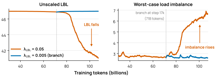
Figure 42. The load-balancing loss falls while load imbalance rises. Interactive adaptation. The full report caption accompanies the original figure.
A direct requested-load metric used by Olmo is the maximum expert count divided by the mean expert count. It is the expert-level instance of Equation 22: \[ I_{\max}^{\mathrm{req}} \mathrel{:\mkern-0.25mu=}\frac{\max_i C_i}{\frac{1}{N}\sum_i C_i} = N\max_i f_i. \tag{39} \] Perfect requested balance gives \(I_{\max}^{\mathrm{req}}=1\). The number of never-selected experts, the coefficient of variation of the \(C_i\), and the sum of counts placed on each expert-parallel rank provide complementary views. Requested counts determine demand; capacity converts demand into the kept counts that determine expert compute and actual communication.
The Switch-style loss in Equation 30 instead couples the hard and soft vectors. Olmo constructs \(C_i^{\mathrm{req}}\) from top-\(K\) indices before capacity under no-gradient bookkeeping and differentiates Equation 30 only through \(P_i\). For sigmoid routing, the scores used by this loss are normalized across experts before the dot product, so the analysis below applies to both normalized sigmoid and softmax scores.
The standard presentation associates the minimum of this objective with uniform requested and soft routing (Fedus et al. 2022, sec. 2.2 and Appendix F). That conclusion would follow immediately if one could identify the soft proxy with requested load. If \(\boldsymbol{P}=\boldsymbol{f}\), then \[ \mathcal{L}_{\mathrm{LBL}} = N\lVert\boldsymbol{f}\rVert_2^2 = 1 + N\lVert\boldsymbol{f}-\boldsymbol{u}\rVert_2^2, \qquad u_i\mathrel{:\mkern-0.25mu=}\frac{1}{N}, \tag{40} \] and uniform requested load is the unique minimizer. Top-\(K\) routing does not impose \(\boldsymbol{P}=\boldsymbol{f}\). It imposes only an ordering constraint within each token: selected experts must outrank unselected experts. Aggregating those token-wise inequalities does not make the two expert-wise marginals equal.
10.7.2 The Centered Form Exposes the Surrogate
Let \(\boldsymbol{u}=(1/N,\ldots,1/N)\) be uniform load. Because both \(\boldsymbol{f}-\boldsymbol{u}\) and \(\boldsymbol{P}-\boldsymbol{u}\) sum to zero, expanding Equation 30 gives \[ \boxed{ \mathcal{L}_{\mathrm{LBL}} = 1 + N(\boldsymbol{f}-\boldsymbol{u})^{\mathsf T} (\boldsymbol{P}-\boldsymbol{u}) = 1 + N^2 \operatorname{Cov}_{i\sim\operatorname{Unif}([N])}(f_i,P_i). } \tag{41} \] Here the covariance is taken across expert coordinates within one balance scope. It is not a stochastic claim about correlation over training time.
In Equation 41, if the hard and soft deviations point in the same direction, the centered inner product is positive and the loss exceeds one. If either vector is uniform, or if their deviations are orthogonal, the loss equals one. If the deviations are anti-aligned, the loss is below one. In particular, \[ \boldsymbol{P}=\boldsymbol{u} \quad\Longrightarrow\quad \mathcal{L}_{\mathrm{LBL}}=1 \quad\text{for every probability vector }\boldsymbol{f}. \tag{42} \] With deterministic tie breaking, uniform scores can pair exactly with a collapsed requested-route histogram; with strict routing margins, that pair can be approached arbitrarily closely by giving the winning expert an infinitesimal advantage. Thus collapse can have the same limiting scalar value as perfect balance. More strongly, the compatible anti-aligned constructions below score better than perfect balance.
The scalar thus fails as a balance metric even though its stop-gradient construction can still push score mass away from frequently selected experts. Liu (2024) gave a compatible one-dead-expert counterexample in which the scalar falls below one, while Su (2025) emphasized that the scalar value and its balancing gradient are different objects. In peer-reviewed work, Lange et al. (2026) identified a related blind spot in which global-batch LBL can appear balanced even when some experts remain barely used. The centered form makes that blind spot exact: Equation 30 controls one signed cross-term, but it controls neither \(\lVert\boldsymbol{f}-\boldsymbol{u}\rVert_2\) nor \(\lVert\boldsymbol{P}-\boldsymbol{u}\rVert_2\) separately. The following constructions quantify how far the scalar can fall below one under imbalanced routing.
10.7.3 A Six-Token Counterexample
The smallest useful example has two experts, top-1 routing, and six tokens. No capacity filter is present, so requested and kept routes coincide. Ignore the batch dimension and use the normalized score matrix \[ \begin{bmatrix} 1.0 & 0.0 \\ 1.0 & 0.0 \\ 0.4 & 0.6 \\ 0.4 & 0.6 \\ 0.4 & 0.6 \\ 0.4 & 0.6 \end{bmatrix}. \tag{43} \] Expert 1 wins the first two tokens, while expert 2 wins the other four. The requested hard and soft marginals are \[ \boldsymbol{C}^{\mathrm{req}}=(2,4), \qquad \boldsymbol{f}=\left(\frac{1}{3},\frac{2}{3}\right), \qquad \boldsymbol{P}=\left(\frac{3}{5},\frac{2}{5}\right). \tag{44} \] The requested imbalance is \(I_{\max}^{\mathrm{req}}=4/3\), yet \[ \mathcal{L}_{\mathrm{LBL}} = 2\left( \frac{1}{3}\frac{3}{5} + \frac{2}{3}\frac{2}{5} \right) = \frac{14}{15} \approx 0.9333 < 1. \tag{45} \]
Panels (a) and (b) of Figure 43 recast the six-token example as equal winner-take-all “elections.” Both panels hold \(\boldsymbol{P}=(3/5,2/5)\) fixed; moving from the hard-balanced panel (a) to panel (b) changes the requested route fraction from \((1/2,1/2)\) to \((1/3,2/3)\). The same soft mass is packed into two decisive expert-1 wins while expert 2 wins four by smaller margins; the requested expert load becomes less balanced as the auxiliary scalar falls from one to \(14/15\).
Figure 43Interactive · conceptual, the report’s exact score tables · not training data
Same soft mass, different winners: move the scores and watch the scalar
Edited your score table
(b) Token Gerrymandering Two 10:0 wins for A; four 40:60 wins for B
- Expert 1 (A)
- Expert 2 (B)
- border = selected route
- T11.0 : 0.0
A wins
- T21.0 : 0.0
A wins
- T30.4 : 0.6
B wins
- T40.4 : 0.6
B wins
- T50.4 : 0.6
B wins
- T60.4 : 0.6
B wins
Each dot is one tenth of a token’s normalized score. Use +A / +B, or focus a token and press ↑ / ↓, to move a tenth; a 5:5 token is the ε → 0+ limit, and the next step flips its winner.
Mean soft mass P
Requested route fraction f 2 of 6 tokens choose A
- Requested imbalance Ireqmax
- 4/3 ≈ 1.333
- Unscaled LBL
- = 14/15 ≈ 0.933
lowest any table with this 2:4 split can approach: 1 − x + 2x² = 8/9this tablebelow balanced
Centered form: 1 + 4(fA − ½)(PA − ½) = 1 + 4 × (−0.167) × (+0.100) = 1 − 0.067
“If the deviations are anti-aligned, the loss is below one.”
Section 10.7.2
“The same soft mass is packed into two decisive expert-1 wins while expert 2 wins four by smaller margins; the requested expert load becomes less balanced as the auxiliary scalar falls from one to 14/15.”
Section 10.7.3
Two experts, top-1 routing, no capacity filter. Presets (a)–(c) are the report’s score tables (Equation 43 and the original figure). Every value is computed exactly from the tokens shown: f and P by Equation 38, the imbalance by Equation 39, the scalar by Equation 30, and its centered form by Equation 41. The lower bound for a fixed route split is Equation 48. Edited tables are feasible score tables, not training data.
Original report figure
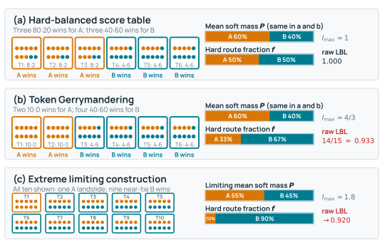
Figure 43. Soft router mass and requested routes can diverge sharply. Interactive adaptation. The full report caption accompanies the original figure.
After aggregation, the lightly loaded expert holds more soft mass and the heavily loaded expert less, so their centered marginals are exactly anti-aligned, the property quantified by Equation 41. The election analogy describes only this concentration of score mass; the tokens themselves stay fixed.
This example disproves any monotonic interpretation of \(\mathcal{L}_{\mathrm{LBL}}\) as requested-route imbalance: a lower value coexists with a higher value of the direct requested-load metric. It is not itself an optimum. The next result shows that the discrepancy is a global score-level property rather than an isolated numerical choice.
10.7.4 Perfect Balance Is Not the Global Score-Level Optimum
For two experts and top-1 routing, relabel the underloaded expert as expert 1 and write \[ \boldsymbol{f}=(x,1-x), \qquad 0\leq x\leq\frac{1}{2}. \tag{46} \] For one token, let \(q\) be its soft probability for expert 1. The token’s contribution to \(\boldsymbol{f}^{\mathsf T}\boldsymbol{p}_t\) is \[ xq+(1-x)(1-q) = (1-x)+(2x-1)q. \tag{47} \] Since \(2x-1\leq0\), this quantity decreases as \(q\) increases. On the fraction \(x\) of tokens routed to expert 1, the smallest contribution is approached by \(q\to1\), giving contribution \(x\). On tokens routed to expert 2, top-1 routing requires \(q<1/2\); the smallest contribution is approached by \(q\to1/2\) from below, giving contribution \(1/2\). Therefore, for a fixed requested load \(x\), \[ \inf \mathcal{L}_{\mathrm{LBL}}(x) = 2\left[x\cdot x+(1-x)\frac{1}{2}\right] = 1-x+2x^2. \tag{48} \] Differentiating the final quadratic gives its minimum at \(x=1/4\): \[ \inf_{x,\{\boldsymbol{p}_t\}} \mathcal{L}_{\mathrm{LBL}} = \frac{7}{8}, \qquad \boldsymbol{f}=\left(\frac{1}{4},\frac{3}{4}\right). \tag{49} \] Thus the global score-level infimum has a 1:3 requested-load split, whereas perfect balance has value one. For the fixed 2:4 split in Equation 44, the infimum is \(8/9\); replacing the four \((0.4,0.6)\) rows by \((1/2-\epsilon,1/2+\epsilon)\) approaches that value.
The result is an infimum: a finite softmax cannot produce an exact zero or one, and strict top-1 assignment approaches the overloaded expert’s tie from one side. Finite \(T\) also discretizes \(x\). The result concerns free per-token normalized score tables with compatible requested counts; it does not claim that every shared linear router attains a smooth finite-logit minimum. A balanced positive-margin assignment is a flat, non-strict local plateau with value one while its requested assignments remain unchanged; it is simply not the global score-level optimum.
10.7.5 Token Gerrymandering Scales to Many Experts
The two-expert gap is bounded, but the same mechanism becomes much stronger with many experts. Choose \(A\) active experts and \(D=N-A\) dead, or never-selected, experts. Route tokens uniformly among the active experts, so an active expert has \(f_j=1/A\) and a dead expert has \(f_d=0\). For \(0<\epsilon<1\), on a token routed to active expert \(j\), choose the limiting score pattern \[ p_{t,j}=\frac{1+D\epsilon}{D+1}, \qquad p_{t,d}=\frac{1-\epsilon}{D+1} \ \text{for every dead expert }d, \qquad p_{t,r}\to0 \ \text{for other active experts }r, \tag{50} \] then take \(\epsilon\to0^+\). These scores sum to one in the zero-tail limit, and expert \(j\) beats every dead expert by \(\epsilon\). The dead experts collectively absorb almost all soft mass, but none is selected. An active expert wins only \(1/A\) of the tokens, so \[ P_j\longrightarrow\frac{1}{A(D+1)} \quad\Longrightarrow\quad \mathcal{L}_{\mathrm{LBL}} \longrightarrow \frac{N}{A(N-A+1)}. \tag{51} \]
For \(N=64\) and \(A=16\), the limiting loss is \(64/(16\cdot49)\approx0.0816\), even though 48 experts are dead and \(I_{\max}^{\mathrm{req}}=\tfrac{N}{A}=4\). Choosing \(A\approx(N+1)/2\) makes the constructed value approximately \(4/N\) while roughly half the experts are unused. An even sharper asymptotic comparison takes \(A\approx\sqrt{N}\): then \(\mathcal{L}_{\mathrm{LBL}}=O(N^{-1/2})\) approaches zero while \(I_{\max}^{\mathrm{req}}=\Theta(N^{1/2})\) diverges and almost every expert is dead. These are feasible limiting constructions, not claims about the typical route distribution of a trained model. Figure 44b plots this family over the full range of \(A\).
The construction also extends to top-\(K\). Select each token’s \(K\) winners uniformly from \(A\geq K\) active experts. For \(0<\epsilon<1/K\), give each winner score \((1+D\epsilon)/(D+K)\), each dead expert score \((1-K\epsilon)/(D+K)\), and the other active experts scores approaching zero, then take \(\epsilon\to0^+\). Every active expert has \(f_j=1/A\) and \(P_j\to K/[A(D+K)]\), yielding \[ \mathcal{L}_{\mathrm{LBL}} \longrightarrow \frac{NK}{A(N-A+K)}. \tag{52} \] The construction upper-bounds the general score-level infimum and is enough to refute uniform global optimality. We do not claim that Equation 52 is the exact optimum for arbitrary \((N,K,T)\), tie breaking, grouped selection, or score-correction bias.
Figure 44Interactive · conceptual, the report’s closed-form constructions · no training measurements
Slide the route split and the active-expert count: the scalar can prefer imbalanced routes
(a) Two experts, top-1 Equation 48
x = 0.250route split 25.0% : 75.0%Ireqmax = 2(1 − x) = 1.500inf LBL = 1 − x + 2x² = 0.8750
Requested route fraction f expert 1 underloaded
Limiting soft mass P expert-1 routes score (1, 0); expert-2 routes score (½−ε, ½+ε)
(b) Many experts, A active Equation 51 · Equation 52
16 active · 48 deadIreqmax = N/A = 4LBL → 4/49 = 0.0816
Dead experts hold 98.0% of the soft mass and win no route.
The report’s panel: N = 64, top-1. Experts are ordered active first; bars share one scale.
Both panels evaluate the report’s closed forms: (a) the fixed-load score-level infimum of Equation 48, with its marked points from Equation 49 and the six-token example; (b) the limiting value of the explicit construction, Equation 51 for top-1 and Equation 52 for top-K. Other N and K values evaluate the same equations; they are feasible limiting constructions, not optima for arbitrary (N, K, T) and not route distributions of a trained model.
Original report figure
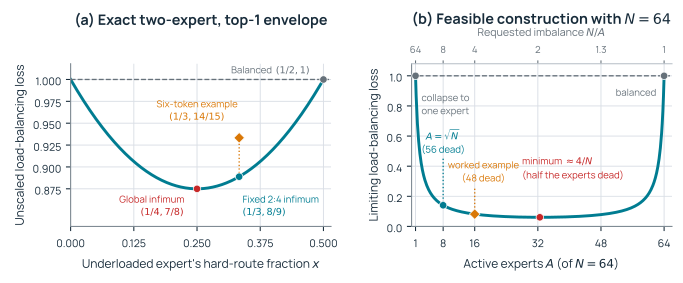
Figure 44. The Switch-style scalar can prefer imbalanced requested routes. Interactive adaptation. The full report caption accompanies the original figure.
The many-expert construction preserves the same requested-load/soft-mass anti-alignment as the two-expert example.
10.7.6 A Larger Scope Does Not Repair the Surrogate
Changing the balance scope leaves the scalar’s limitation intact. For any scope in which \(\boldsymbol{f}\) and \(\boldsymbol{P}\) are normalized over the same tokens, Equation 41 still holds. A global-batch LBL gives the router more tokens over which to satisfy the constraint; it does not turn \(N\boldsymbol{f}^{\mathsf T}\boldsymbol{P}\) into a norm of global requested load. Instance-level balancing prevents cancellation between sequences, but it does not remove the anti-alignment construction within one sequence. Likewise, synchronized-microbatch, online-global, and exact optimizer-batch statistics change which tokens may compensate for one another without changing the signed cross-term itself.
10.8 Gradient Dynamics and the Joint Objective
The requested counts are detached, so within a region where top-\(K\) assignments do not change, \(\boldsymbol{f}\) is constant. For top-1 softmax logits \(z_{t,i}\), differentiating Equation 30 gives \[ \frac{\partial\mathcal{L}_{\mathrm{LBL}}}{\partial z_{t,i}} = \frac{N}{T}p_{t,i} \left(f_i-\boldsymbol{f}^{\mathsf T}\boldsymbol{p}_t\right). \tag{53} \] For every token, the auxiliary gradient transfers soft mass toward experts whose requested load \(f_i\) is below the score-weighted average. This is the intended balancing pressure. A task-preferred, frequently selected expert can nevertheless remain the winner by an arbitrarily small margin while cold or dead experts absorb much of the differentiable mass. The gradient can therefore improve the surrogate faster than it improves the requested-selection histogram.
Routing boundaries make the dynamics discontinuous. When two scores cross, the hard vector \(\boldsymbol{f}\) changes abruptly and the gradient field is recomputed. A shared router may cross, cycle around, or avoid the limiting score tables above. The theory establishes feasible objective geometry; by itself it does not prove that stochastic gradient descent reaches a stable gerrymandered routing pattern.
The connection to training appears only after restoring the auxiliary coefficient. Write the optimized objective as \[ \mathcal{L}_{\mathrm{train}} = \mathcal{L}_{\mathrm{CE}} + \lambda_{\mathrm{LBL}}\mathcal{L}_{\mathrm{LBL}} + \mathcal{L}_{\mathrm{other}}, \tag{54} \] where \(\mathcal{L}_{\mathrm{CE}}\) is next-token cross-entropy (CE) and \(\mathcal{L}_{\mathrm{other}}\) contains every other enabled term, such as a router z-loss (Zoph et al. 2022) or language-model z-loss (Chowdhery et al. 2023). Compare the model before and after a routing transition on the same evaluation batch with fixed loss normalization. If the transition hurts language modeling but reduces LBL, then \[ \Delta\mathcal{L}_{\mathrm{CE}}>0, \qquad \Delta\mathcal{L}_{\mathrm{LBL}}<0. \tag{55} \] The post-transition model has a lower scalar objective exactly when \[ \Delta\mathcal{L}_{\mathrm{train}}<0 \quad\Longleftrightarrow\quad \lambda_{\mathrm{LBL}} \left(-\Delta\mathcal{L}_{\mathrm{LBL}}\right) > \Delta\mathcal{L}_{\mathrm{CE}} + \Delta\mathcal{L}_{\mathrm{other}}. \tag{56} \] Whether an LBL coefficient is high depends on the net CE and other-term cost of a reachable routing transition, the number of routed layers contributing auxiliary loss, and the implementation’s layer and microbatch normalization; there is no universal numerical threshold. A larger coefficient does not change the minimizers of LBL alone; it changes which compromises lower the joint objective. When such a compromise wins, the observable pattern is the surrogate-hacking signature: the optimized objective falls while both language-modeling loss and requested imbalance worsen. This before-and-after comparison is not an optimizer-dynamics theorem: momentum and stochastic gradients need not lower the instantaneous loss of every training batch, and losses from different batches do not define the deltas above.
10.8.1 Empirical Signature of Reachable Collapse
The score-level constructions do not show that stochastic training reaches a gerrymandered routing pattern. Figure 45 provides a checkpoint-branched test in a 48-layer, 64-expert, top-4 MoE. The original trajectory uses instance-level LBL with \(\lambda_{\mathrm{LBL}}=0.05\). At step 17,000 (71.3 billion training tokens), before the observed divergence, a second trajectory reloads the same model and optimizer checkpoint and changes the coefficient to \(0.005\). This intervention controls the starting point more tightly than an independent-from-scratch coefficient sweep. Dispatch is dropless in these runs, so requested counts are also the executed expert loads. Block 0 is dense, so the logged LBL is the sum of the instance-level loss over the 47 MoE blocks; the logged load imbalance is the worst max/mean expert count over those blocks and distributed ranks. These runs use the production HSDP pretraining stack rather than the expert-parallel paths of this report. Appendix B.7 records the full run recipe and the archived-history provenance.
Figure 45Interactive · measured, one 48-layer, 64-expert, top-4 run · raw values in 20-step ranges
One cursor across three metrics: after the branch, only the high-coefficient run degrades
- λLBL = 0.05 · original
- λLBL = 0.005 · branch from step 17,000
- raw range
- early / late windows
Cross-entropy loss
Worst-case load imbalance worst max/mean expert count over blocks and ranks · dotted: ideal 1
Unscaled LBL sum over 47 MoE blocks · dotted: balanced 47
At 104.0B tokens · step 24,791 · smoothed value, with the raw range over steps 24,781–24,800
Plotted from the report’s archived W&B histories (the plotting table of the original figure). Thick lines are the report’s time-weighted EMA; the light band is the envelope of every raw measurement within 20-step buckets, and the cursor reads one stored 20-step sample. The shaded windows are the steps behind the medians in Table 20. Dispatch is dropless in these runs; Appendix B.7 records the run recipe.
Original report figure
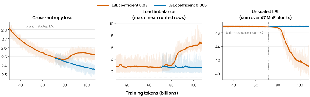
Figure 45. Checkpoint-branched training with different LBL coefficients. Interactive adaptation. The full report caption accompanies the original figure.
The comparison establishes the surrogate–workload mismatch (Table 20). Between the early and late windows, the high-coefficient trajectory lowers its unscaled LBL sum by about twelve percent while its worst-case load imbalance more than doubles and its CE worsens; the low-coefficient branch improves CE while its LBL stays near the balanced reference and its imbalance does not rise. The effect is not isolated to one layer: median imbalance increases in all 47 MoE blocks on the high-coefficient trajectory, and over the branched interval its unscaled LBL and worst-case load imbalance have Spearman correlation \(-0.87\).
| High coefficient (\(\lambda_{\mathrm{LBL}}=0.05\)) | Low-coefficient branch (0.005) | |||||
| Median over window | Early | Late | Change | Early | Late | Change |
| CE loss | 2.473 | 2.523 | +2.0% | 2.469 | 2.358 | −4.5% |
| Unscaled LBL sum | 46.864 | 41.278 | −11.9% | ≈ 47 | ≈ 47 | stable |
| Worst-case load imbalance | 2.748 | 6.317 | +129.9% | 2.655 | 2.544 | −4.2% |
The unscaled LBL and CE curves in Figure 45 have different weights in the optimized objective. Figure 46 combines them with those weights for the high-coefficient trajectory.
Figure 46Interactive · measured, λ = 0.05 trajectory only · objective reconstructed from logged terms
Take the objective apart: weighted LBL falls faster than CE rises
- Total objective
- CE
- Weighted LBL (0.05 × unscaled)
Each curve minus its early-window median (total 4.820, CE 2.473, weighted LBL 2.343).
At 104.0B tokens step 24,791 · smoothed, λLBL = 0.05
Early → late window medians: CE and LBL from Table 20, weighted LBL and total from the text
Weighted LBL falls by 0.279 = 0.05 × (46.864 − 41.278); CE rises by 0.050. Total −4.8%.
Medians of training-batch measurements, so the parts need not add exactly. Router z-loss is disabled in these runs.
Plotted from the report’s archived training metrics. Black, purple and green are the total and its components, not coefficient settings. The total is the report’s reconstruction: logged CE plus coefficient-weighted LBL plus the enabled LM-head z-loss. The window values with the chart are the medians printed in Table 20 and the text; they compare stochastic training batches, not one fixed batch, so they illustrate rather than evaluate Equation 56.
Original report figure
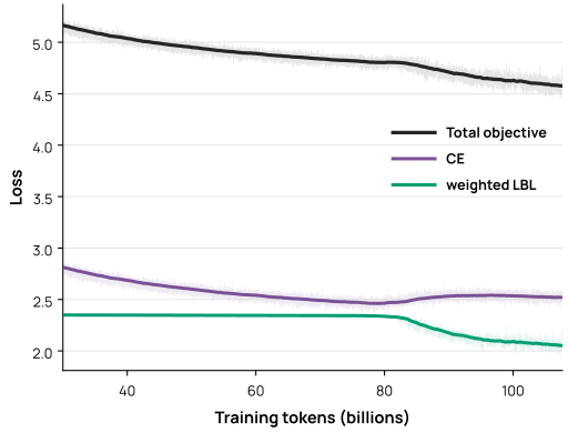
Figure 46. The reconstructed objective decreases despite worsening CE. Interactive adaptation. The full report caption accompanies the original figure.
Over the same windows, the median coefficient-weighted LBL contribution falls from \(2.343\) to \(2.064\), enough for the median reconstructed optimized objective to decrease from \(4.820\) to \(4.591\) (\(-4.8\%\)) despite the CE regression. Olmo injects LBL through a custom autograd term rather than adding it to one monolithic forward-loss scalar. The plotted objective therefore reconstructs the optimized scalar from the separately logged CE, coefficient-weighted LBL, and LM-head z-loss. Router z-loss is disabled in these runs.
This establishes reachability of the predicted surrogate-hacking signature for this configuration: training can lower the effective objective while making both language modeling and routed workload worse. It does not locate a universal coefficient threshold or establish how frequently the failure occurs. These are also stochastic training-batch curves rather than losses reevaluated on one fixed batch, and the archived metrics do not contain same-scope \(\boldsymbol{f}\) and \(\boldsymbol{P}\) vectors. Attributing the trajectory to the exact hard/soft anti-alignment construction would require the centered term in Equation 41, or equivalent evidence from soft mass on never-selected experts and top-\(K\)–top-\((K+1)\) margins. A lower LBL scalar did not certify a more balanced expert workload.
10.9 Measuring Routing Transients and Outcomes
Routing is nonstationary, especially early in training. A router can move from near-random assignments through sharp transients before reaching a more stable distribution, and both capacity utilization and step time can move with it. Uniform or random expert assignment is useful for isolating an optimistic balanced systems path, but it is not a substitute for trained routing. Interpreting throughput therefore requires knowing whether the routes are artificially balanced, early-transient, or drawn from a declared stable training window. Three diagnostic questions connect those routing conditions to the model and systems outcomes.
What did the router request, and what did capacity admit?
\(\boldsymbol{C}^{\mathrm{req}}\) records selected top-\(K\) routes before capacity, and \(\boldsymbol{C}^{\mathrm{keep}}\) records the rows admitted for expert execution. When no route is dropped the two hard histograms coincide. Otherwise both histograms are needed. Route-drop rate, the fraction of tokens losing at least one or all selected routes, selected weight removed by dropping, and receiving-buffer utilization describe how capacity changed the workload and removed model contributions.
Which experts or ranks became bottlenecks?
Max/mean and a full-distribution statistic for requested expert counts, the number of never-selected experts, and the maximum requested load on one expert-parallel rank distinguish expert concentration from rank pressure. The corresponding kept-count statistics describe the work that actually ran. Grouped-GEMM and step time connect kept counts to computation; the source–destination request matrix and rank waiting connect demand and admitted work to communication and straggling.
Did balance improve, or only the surrogate?
The soft mean \(\boldsymbol{P}\) summarizes differentiable router mass rather than selected or executed routes. Diagnosing Token Gerrymandering requires the requested hard fraction \(\boldsymbol{f}\) and soft mean \(\boldsymbol{P}\) from the same routed layer and load-balancing scope. Their centered inner product, together with \(\lVert\boldsymbol{f}-\boldsymbol{u}\rVert_2\) and \(\lVert\boldsymbol{P}-\boldsymbol{u}\rVert_2\), separates anti-alignment from the magnitude of each deviation; top-\(K\)–top-\((K+1)\) margins and soft mass on never-selected experts provide complementary evidence. Pearson correlation alone is insufficient because it is undefined when either vector is uniform and discards the magnitudes that determine LBL.
The effect on the optimized objective depends on the effective LBL contribution after layer and microbatch normalization, together with every enabled auxiliary term. An unscaled LBL curve beside CE can disprove the scalar’s use as a balance certificate, but it cannot establish why the optimizer preferred a transition.
The evidence in this section establishes the objective geometry, the fixed-work grouped-GEMM sensitivity, and the reachability of the surrogate-hacking signature in one checkpoint-branched training comparison. The requested and kept workloads, rather than the auxiliary scalar alone, connect routing to the expert GEMMs and communication that the training system executes.