Section 11: MXFP8 Training

Routing determines which expert GEMMs run and how their work is distributed. MXFP8 changes the precision and volume of the operands those GEMMs compute with and communicate.

Microscaling (MX) formats pair a low-precision payload with one shared power-of-two scale per small block of values; MXFP8 is the member with an FP8 payload and 32-value blocks, standardized by the Open Compute Project (OCP) together with the FP8 payload formats (Micikevicius et al. 2022; Rouhani et al. 2023; Open Compute Project 2023). In training, MXFP8 requires changes to operand quantization, scale layouts, saved activations, expert transport, and weight refresh after each optimizer update. Those changes can accelerate sufficiently large GEMMs, reduce storage for selected saved activations, and shrink expert-communication payloads. They also add conversion, layout, transport-management, caching, and backward work. Section 11.1 quantifies the potential savings and explains why persistent training-state memory stays approximately unchanged.

Blackwell is the main hardware target for the implementation described here. Hopper supports FP8 Tensor Core operations; Blackwell adds native support for the 32-value, E8M0-scaled block representation used by MXFP8 (Open Compute Project 2023; NVIDIA 2026d). The Tensor Core operation can consume quantized operands and their block scales together. Software must still create both components in the layouts expected by the instruction.

Table 21 separates ordinary FP8 support from native MXFP8 support. Hopper accelerates E4M3 and E5M2 FP8, but it does not provide the block-scaled matrix instruction that consumes an E8M0 scale per 32 payload values. The Blackwell variants in the table do. Their instruction families differ: data-center Blackwell uses tcgen05.mma, while SM120 RTX Blackwell exposes block scaling through mma.sync.

11.1 Benefits of MXFP8 Training

11.1.1 Faster GEMMs

A BF16 GEMM uses two bytes per input value and the BF16 Tensor Core path. The Olmo MXFP8 recipe uses one E4M3 payload byte per value plus block scales, and on Blackwell GPUs it uses the higher-throughput FP8 Tensor Core path. Peak Tensor Core specifications list an exact \(2\times\) FP8-to-BF16 ratio on both Hopper and Blackwell (Table 21) (NVIDIA 2026p, 2026q). That ratio is an arithmetic ceiling, not an end-to-end speedup: quantization (Q), dequantization (DQ), scale construction, layout conversion, kernel launches, small GEMMs, communication, and all non-GEMM work remain on the step timeline.

Figure 47 contrasts the operands supplied to the BF16 and native MXFP8 Tensor Core paths. The BF16 path consumes two BF16 matrices. The MXFP8 path consumes E4M3 qdata together with one E8M0 scale per 32 values along the reduction dimension. On Blackwell, the instruction-level primitive is a fifth-generation Tensor Core matrix multiply–accumulate (MMA): the MXFP8 path uses the block-scaled tcgen05.mma family. The scale shapes in the figure are the logical pre-swizzle grids; the physical blocked layouts consumed by the instruction are more specialized. Appendix A.5 separates the PyTorch operator, GEMM kernel, and Tensor Core instruction interfaces in more detail.

Figure 47Interactive · conceptual operand structure, no timing

Pick an output element: which qdata and scales feed it?

Tensor Core path

BF16Native MXFP8

Shape for the byte count

4096 → 4096OLMoE 1536 → 307216384 → 2048

• E4M3 qdata · 1 B/value
• E8M0 scale · 1 per 32 values along K
• BF16 · 2 B/value

Cell area is proportional to bytes: BF16 2 B/value · E4M3 1 B/value · E8M0 scale chips (1 B per 32 values) enlarged to stay visible

Conceptual diagram of the logical, pre-swizzle scale grids (Figure 52 shows the physical layout). Point at, tap or tab to an output element, an operand block, a scale or a stage of the operator. Byte counts are nominal arithmetic for the chosen shape, not measurements.

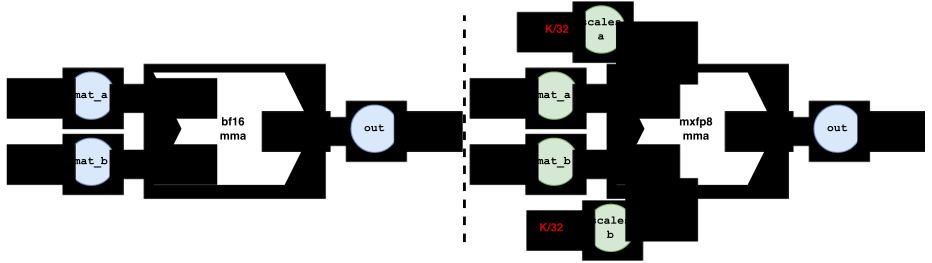
Figure 47. BF16 and native MXFP8 Tensor Core paths. For \(A\in\mathbb{R}^{M\times K}\) and \(B\in\mathbb{R}^{K\times N}\), the MXFP8 operation consumes E4M3 qdata and logical scale grids of shape \(M\times(K/32)\) and \((K/32)\times N\) before scale swizzling. “MMA” names the native Tensor Core operation accurately: Blackwell provides tcgen05.mma instructions with the kind::mxf8f6f4 and block_scale modifiers for this computation. Olmo invokes the higher-level scaled_mm operator, whose kernel includes the MMA main loop and an epilogue that converts the accumulator to the requested BF16 output. Thus, BF16 labels the completed operator output, not the raw MMA accumulator.

The attainable speedup depends on shape. Large dense GEMMs can amortize operand quantization and scale-layout work over substantial matrix multiplication. A routed layer may instead present many smaller expert GEMMs, where the same fixed work occupies a larger fraction of kernel time. Weight quantization is easier to amortize because its caches are rebuilt after an optimizer update and reused across the following microbatches. Activation quantization is paid on each invocation.

11.1.2 Smaller Saved Activations

For a block of 32 values, the nominal MXFP8 representation contains 32 bytes of E4M3 qdata and one byte of E8M0 scale. Ignoring blocked-layout padding, its storage per value is

\[ B_{\mathrm{MXFP8}} = 1 + \frac{1}{32} = \frac{33}{32} \quad\text{bytes/value}, \tag{57} \]

compared with two bytes per BF16 value. Replacing a unique BF16 saved tensor with this representation saves \(31/32\) bytes per value, a nominal reduction of \(1-33/64\approx48.4\%\). If another operator already keeps the same BF16 activation alive, adding an MXFP8 copy instead costs another \(33/32\) bytes per value. The implementation must therefore determine whether another operator already retains each BF16 tensor before choosing its saved precision. In our attention path, for example, the QKV projection and output projection use different save policies because their BF16 inputs are retained by different parts of the backward graph. Figure 58 (Section 11.4) shows the resulting boundary between forward-time packing and backward-time unpacking.

11.1.3 Smaller Dispatch and Combine Payloads

Rowwise EP normally moves one hidden row for each routed token–expert assignment. A BF16 row of width \(d\) carries \(2d\) payload bytes. When \(d\) is a multiple of 32, its nominal MXFP8 representation carries \(d+d/32=33d/32\) bytes, again a \(48.4\%\) reduction in the row payload.

This does not halve the whole communication operation. Route indices, route weights, counters, and synchronization are unchanged. Qdata and scales also need destinations and transfers of their own. MXFP8 reduces the numerical payload for dispatch and combine, and that reduction is useful when the saved transport time exceeds the added quantization, scale, and transfer-management work.

11.1.4 Persistent Training-State Memory

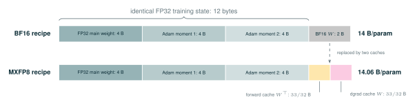
Each linear weight is consumed in two orientations. Forward computes with \(W^\top\), while dgrad computes with \(W\). Each orientation needs its own qdata and scale layout. We call these qdata-and-scale representations MXFP8 compute-weight caches, or simply weight caches in this section. At nominal storage, the two MXFP8 views require \(2\times33/32=2.0625\) bytes per original weight value. This is \(3.125\%\) more than one two-byte BF16 compute weight even before blocked-scale padding.

Our optimizer also retains an FP32 main weight and FP32 optimizer states. After the MXFP8 caches have been initialized, the full BF16 initialization anchor can be released, but the two caches take its place. MXFP8 therefore does not remove the persistent training-state memory wall by itself. EP, PP, and distributed optimizer sharding remain responsible for dividing parameters, gradients, and optimizer tensors, as described in Part II.

Figure 48 compares the two recipes. MXFP8 replaces a two-byte BF16 compute weight with two cache orientations of nearly the same combined size, so the composition of persistent training state changes while its total stays approximately constant.

Figure 48Interactive · conceptual nominal bytes, no measured quantities

The composition changes; the total barely moves

View

Whole stateZoom to the compute weights

Nominal accounting from Section 11.1.4 and the figure caption: 4-byte FP32 main weight and Adam moments, a 2-byte BF16 compute weight, and two MXFP8 weight caches at 33/32 bytes each. MXFP8 does not shrink this persistent state; EP, PP and distributed-optimizer sharding divide it.

Figure 48. Persistent memory with BF16 weights and two MXFP8 weight caches. Nominal bytes per parameter: both recipes keep the FP32 main weight and two FP32 Adam moments; the BF16 recipe adds one two-byte compute weight, while the MXFP8 recipe replaces it with the forward and dgrad weight caches at \(33/32\) bytes each. Gradient buffers are identical in both recipes and excluded, and blocked-scale padding is ignored. Conceptual illustration of the nominal accounting with no measured quantities.

11.2 Understanding the MXFP8 Format

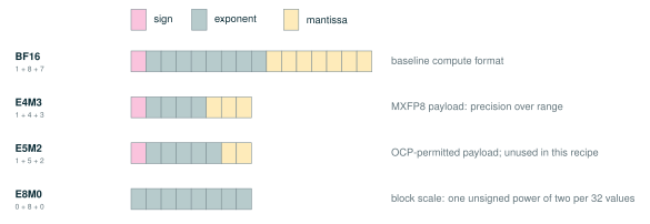
An MXFP8 tensor is defined by more than its one-byte E4M3 payload. Its E8M0 scales, the number of payload values that share each scale, and the physical scale layout consumed by a particular operand role are equally important. These details explain why conversion has separate quantization and swizzle costs, why qdata and scales cross operator boundaries together, and why native MXFP8 GEMM requires Blackwell-specific hardware support. Figure 49 compares the bit layouts involved: the BF16 baseline, the two payload formats the OCP MX specification permits, and the E8M0 scale.

Figure 49Interactive · conceptual format arithmetic, no measured quantities

Type a value, or flip a bit: what does each format keep?

Value x

Try

0.31448E4M3 max5000.001−2.75

Each format below shows how it stores x, using round-to-nearest-even and saturation at its largest finite value; E8M0 keeps only the power of two.

signexponentmantissaSelect a bit to flip it; arrow keys move between bits

BF161 + 8 + 7

0011111010011010

0.300781250x3E9A · rel. error 0.26%

baseline compute format

E4M31 + 4 + 3

00101010

0.31250x2A · rel. error 4.2%

MXFP8 payload: precision over range

E5M21 + 5 + 2

00110101

0.31250x35 · rel. error 4.2%

OCP-permitted payload; unused in this recipe

E8M00 + 8 + 0

01111101

2⁻² = 0.250x7D · rounded down to a power of two; the rceil block scales round up

block scale: one unsigned power of two per 32 values

Representable magnitudes log₂ scale; light = subnormal; the pink line is |x|

Range and spacing of each format

Format	Exponent / mantissa bits	Largest finite	Smallest normal	Smallest subnormal	Spacing just above 1
BF16	8 / 7	3.39 × 10³⁸	2⁻¹²⁶	2⁻¹³³	2⁻⁷ = 0.0078125
E4M3	4 / 3	448	2⁻⁶ = 0.015625	2⁻⁹ = 0.00195313	2⁻³ = 0.125
E5M2	5 / 2	57344	2⁻¹⁴ = 6.104 × 10⁻⁵	2⁻¹⁶ = 1.526 × 10⁻⁵	2⁻² = 0.25
E8M0	8 / 0	2¹²⁷	2⁻¹²⁷	none	×2 (powers of two only)

Conversions round to nearest even and saturate at the largest finite value, as in the report’s pseudocode (Table 24). E5M2 is shown with the same saturating conversion. Values follow from the bit layouts in the figure (OCP MX v1.0); they are not measurements.

Figure 49. Bit layouts of the baseline, payload, and scale formats. BF16 keeps eight exponent bits and seven mantissa bits. The E4M3 payload trades exponent range for mantissa precision; E5M2 makes the opposite trade and is permitted by OCP MX but unused in the Olmo recipe. The E8M0 scale is an exponent-only format: one unsigned power of two per 32-value block, with no sign and no mantissa.

11.2.1 Quantization, Dequantization, and Swizzle

For a BF16 block \(x\), quantization selects a power-of-two scale \(s\) and stores

\[ q = \operatorname{E4M3}(x/s), \qquad \widehat{x} = s q. \tag{58} \]

The qdata \(q\) and the scale \(s\) together encode one MXFP8 tensor; neither part is usable alone. Dequantization applies the second relation when an operator requires BF16 or FP32 values (Figure 50).

Figure 50Interactive · illustrative example values, not training data

Quantize one 32-value block, then rebuild it: x̂ is close to x, not equal

Block

Smooth blockOne large valueMixed magnitudes

Scale

rceil sOlmos ÷ 2s × 256

Value 23 of 32 through Equation 58

x · BF16

2.28125

x / s = 292

quantize

q · E4M3 qdata

288

0 1111 001

s · E8M0 scale

2⁻⁷

byte 120 = e + 127

dequantize

x̂ = s·q

2.25

error −1.4%

Illustrative block of 32 values, rounded to BF16. Quantization follows the rceil path of Table 24 (the Olmo default): one power-of-two scale s for the block, then saturating round-to-nearest-even into E4M3. The “s ÷ 2” and “s × 256” buttons override that choice only to show its effect: a smaller scale saturates the largest values, a much larger one leaves small values subnormal or flushes them to zero. Point at, tap or use the arrow keys to follow one value.

Figure 50. Quantization produces a qdata–scale pair. Dequantization consumes both components and reconstructs \(\widehat{x}=s q\), an approximation to the original \(x\); it does not invert quantization exactly.

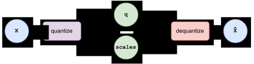
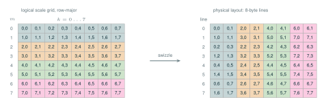
The scale order associated with adjacent 32-value input blocks is not necessarily the blocked order required by a GEMM. Scaled matrix-multiply kernels consume swizzled scale layouts chosen for Tensor Core access. Quantization therefore has two distinct tasks: compute the scale and qdata, then arrange the scales for the operand role and matrix layout used by the kernel. Rowwise communication may use a different addressable scale layout from scaled GEMM (NVIDIA 2026w). Figure 51 draws the block decomposition, and Figure 52 draws the layout distinction.

Figure 51Interactive · conceptual, drawn to byte scale, no measured quantities

Two contiguous arrays: where each block’s qdata and scale go

Rows

2report4

Blocks per row

2report4

Scales

True widthMagnify ×8

Point at, tap or tab to a block to see where its bytes live. Arrays are contiguous; the dashed spans are logical.

Widths are proportional to bytes: a BF16 block is 64 B, its E4M3 qdata block 32 B, and its E8M0 scale 1 B. Colors mark which block each scale covers. Blocked-layout padding is ignored, as in Equation 57.

Figure 51. Quantization produces one contiguous qdata array and one contiguous scale array. Sizes are drawn to byte scale for a two-row tensor with two 32-value blocks per row: each 64-byte BF16 block becomes a 32-byte E4M3 qdata block, half as wide, and the flattened scale array adds one E8M0 byte per block, each scale \(1/32\) the width of a qdata block. The four scales are the narrow strip at the lower left, drawn at true width; color marks which block each scale covers, and the dashed spans are logical: neither array is fragmented. Conceptual illustration with no measured quantities.

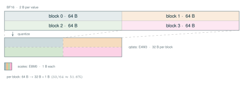
Figure 52Interactive · conceptual layout rule, no measured quantities

Swizzle the scales: sub-blocks move, identities stay

Show

Miniature (as drawn)Hardware rule · 128 × 4 tile

LogicalPhysical

Sub-blocks moved

0 / 16

Follow

Sub-blockRow

Row m

37

Column k

0123

Full-size diagram · labels stay readableSwipe →

The miniature uses two-row groups and two-column tiles, as in the original figure; the hardware rule applies the same relocation with 32-row groups and four-column tiles (128 × 4 scales per 512-byte tile).

Figure 52. The scale order a GEMM consumes is a tiled, interleaved layout. Cells are labeled \(m,k\) for the scale of row \(m\) and block column \(k\), and colors mark row groups. Before the swizzle the grid is row-major; after it, each physical line interleaves the four row groups while a row’s scales within a tile stay adjacent. The drawing is a structure-preserving miniature with two-row groups and two-column tiles; the hardware layout applies the same rule with 32-row groups and four-column tiles, rearranging \(128\times4\) tiles of scales into 32 sixteen-byte lines so that rows \(m\), \(m{+}32\), \(m{+}64\), and \(m{+}96\) become physically adjacent (NVIDIA 2026d). The result resembles a transpose because whole row-group sub-blocks are relocated from a vertical stack to a horizontal line, but it is not one: inside every sub-block, \(m\) still advances downward and \(k\) rightward, and each scale keeps its \(m,k\) identity; only its address changes. Conceptual illustration with no measured quantities.

11.2.2 Scaling Granularity

The number of values sharing a scale affects both numerical precision and storage cost. A tensor-wide scale is cheap to store but must cover the largest value in the tensor. Per-row or per-channel scales track variation more closely at greater metadata and conversion cost. Block scaling lies between those choices. The OCP MX specification permits E4M3 and E5M2 payload formats. Olmo uses the E4M3 MXFP8 variant: each adjacent block of 32 E4M3 values shares one power-of-two E8M0 scale (Open Compute Project 2023). Figure 53 contrasts the three granularities.

Figure 53Interactive · illustrative example values, not training data

One large value sets the scale for its whole group

Scale granularity

Tensor-wide1 scalePer rowM scales32-value blocksM·K/32

One large valueSize

2¹⁴

Illustrative 4 × 64 tensor (typical magnitudes 2⁻⁵ to 2²) and one optional large value in row 1. To isolate the grouping, all three granularities use the same power-of-two rceil scale and E4M3 payload; only the set of values that shares each scale changes. Point at or tap a cell for its numbers; once the tensor has focus, the arrow keys step through the values.

Figure 53. Scale granularity is a spectrum along the reduction dimension. One tensor-wide scale must cover the largest value in the tensor, per-row scales track variation more closely, and 32-value block scales track it most tightly at the highest metadata cost. Conceptual illustration with no measured quantities.

Smaller scale groups reduce the range that any one scale must cover, but they also increase the number of scales that must be produced, moved, and arranged. The 32-value group is therefore part of both the numerical recipe and the systems interface. Shape divisibility and scale layout are not optional kernel details.

11.2.3 Native Blackwell MXFP8 GEMM

Native block scaling applies the E8M0 scales inside the matrix operation (NVIDIA 2026d), avoiding a separate materialization of dequantized operands before GEMM. It accelerates the scaled matrix multiplication itself; software still determines how often values are converted into and out of MXFP8. Those conversions are the first challenge examined in Section 11.3.

11.3 Challenges in MXFP8 Training

Around the native block-scaled GEMM, the training system must produce correctly oriented operands for forward, dgrad, and Wgrad; pass qdata and scales through autograd; refresh derived weight caches after each optimizer update; and avoid paying Q, DQ, or scale swizzles more often than necessary. The following challenges determine whether the hardware throughput advantage survives in end-to-end training.

11.3.1 Quantization and Layout Overhead

For one candidate GEMM (Figure 54), MXFP8 is faster only when

\[ T_{\mathrm{Q}} + T_{\mathrm{layout}} + T_{\mathrm{MXFP8\ GEMM}} + T_{\mathrm{DQ}} < T_{\mathrm{BF16\ GEMM}}. \tag{59} \]

Figure 54Interactive · measured, single-B300 sweep · original figure is a schematic

Does the GEMM saving pay for the conversion? Scrub M and read Equation 59

Projection K → N

1K→1K2K→2K4K→4K4K→6K4K→8K8K→4K2K→16K16K→2K

Rows M

16,384

T_Q + T_layout + T_{MXFP8 GEMM} + T_DQ < T_{BF16 GEMM}

Cached weight: 215 µs < 306 µs → faster than BF16 (1.42×)

On the cached-weight path T_Q is the LHS quantization only (the RHS cache is reused), and the scaled GEMM returns BF16, so no separate DQ kernel runs.

“Not every term is present on every path.”

Section 11.3.1

LHS Q + swizzle, timed alone

117 µs (0.38× the BF16 GEMM)

LHS Q · swizzle, each alone

85.2 µs · 42.7 µs

RHS Q + swizzle (paid at cache refresh)

131 µs

LHS DQ, reported separately

75.7 µs (not invoked by native scaled GEMM)

Measured on one NVIDIA B300 (the report’s single-B300 sweep: M = 128 to 16,384; three warm-ups, then the median of five timed repeats; eager timing, so short calls include submission gaps). Path bars are whole-operation timings; the lighter tail is the path time minus the MXFP8 GEMM time. Component kernels were timed separately and do not add up to a path. The original figure is a schematic of the same inequality; Table 22 gives the crossover points.

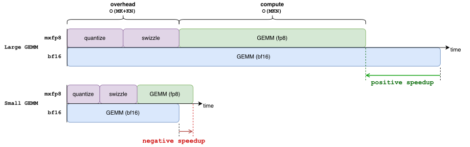
Figure 54. Conversion and layout costs in MXFP8 execution. Interactive adaptation. The full report caption accompanies the original figure.

Not every term is present on every path. A cached weight avoids Q on each microbatch, and a scaled GEMM that returns BF16 may not need a separate output DQ kernel. A saved activation or communicated row requires Q when it is produced and DQ if its consumer requires BF16. These costs are absent from the Tensor Core peak ratio.

The crossover depends on the matrix dimensions and on expert load. Dense linears usually produce a few large GEMMs; MoE grouped GEMMs divide tokens across experts and can become too small or uneven to amortize conversion and launch overhead. Our single-GPU microbenchmark sweeps these dimensions to locate the crossover.

Prequantized MXFP8 overtakes BF16 at smaller sizes than conversion-inclusive execution. Small square projections do not recover the conversion cost within the single-B300 sweep. Table 22 separates the measured crossover points for prequantized GEMM and cached-weight execution with per-call activation quantization. The sweep also records Q, scale swizzle, Q-plus-swizzle, DQ, and fully dynamic execution alongside the BF16 and MXFP8 GEMMs.

Table 23 answers a different question: it compares operator boundaries at the larger assignment size \(M=32{,}768\), rather than locating crossovers. Charging LHS quantization at the routed boundary narrows every advantage and leaves the \(1024\) and \(2048\) squares and the OLMoE-family down projection slower than BF16.

Submission overhead also separates measured kernel work from eager wall time. CUDA-Graph timing shows that Python submission gaps can dominate short eager sequences; removing those gaps measures device-service time, not training wall time. A reported speedup therefore depends on the timing boundary as well as on which conversions it includes.

11.3.2 Forward, Dgrad, and Wgrad Need Different Operands

For a linear layer,

\[ Y=XW^\top, \qquad \nabla_X=\nabla_Y W, \qquad \nabla_W=\nabla_Y^\top X. \tag{60} \]

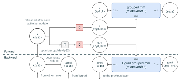
Forward and dgrad use the same weight parameter but opposite matrix orientations. Olmo consequently stores one prequantized RHS cache for \(W^\top\) and another for \(W\). They are derived from one FP32 main weight and must be refreshed together; they are not independent parameters.

The activation has a similar layout problem. In forward, \(X\) is the left-hand operand. In Wgrad, the saved \(X\) is the right-hand operand of \(\nabla_Y^\top X\). The LHS and RHS scale layouts are not interchangeable, so an activation quantized for forward cannot automatically be reused for Wgrad (NVIDIA 2026w). When Olmo saves \(X\) in MXFP8 for Wgrad, it produces the RHS-oriented representation explicitly.

Dense MXFP8Linear uses scaled MXFP8 operations for forward, dgrad, and Wgrad. The current routed grouped-Wgrad path is different: it dequantizes the needed operands and uses BF16 grouped matrix multiplication. The tested natural grouped-Wgrad contraction and scale layouts were slower on the measured development shapes.

Figure 55 draws the resulting weight path: one FP32 main weight quantized after each update into the two oriented caches that forward and dgrad consume. It is a zoom of the full routed pipeline in Figure 57 (Section 11.4) and uses that figure’s notation.

Figure 55Interactive · conceptual weight path, no measured quantities

One FP32 weight, two derived caches: follow one optimizer step

One optimizer step · four microbatches, illustrative

UpdateRefreshF1B1F2B2F3B3F4B4Reduce↺

Refresh caches after each update

Full-size diagramSwipe →

Refresh both caches

Refresh: quantize once into two oriented caches

“After initialization and every optimizer copy-back, Olmo reconstructs the local weight values and rebuilds all required MXFP8 caches.”

Section 11.3.4

“The gather that assembles the sharded main weight stages through a transient BF16 copy freed immediately after quantization”

Figure 55 caption

FP32 main weight

version t+1

Forward cache W

version t+1 current

Dgrad cache W.T

version t+1 current

Weight Q since the update

2

Point at, tap, or tab to a part to read its notation.

Conceptual illustration drawn from the figure’s source. Version labels and the four-microbatch step are illustrative. The dashed transient W (bf16) gather copy is drawn from the caption; the original drawing does not show it.

Figure 55. One FP32 main weight becomes two oriented MXFP8 caches. After every optimizer update, the FP32 main weight is quantized into the forward cache and, through an explicit transpose, the dgrad cache, each consumed as the RHS of its scaled grouped GEMM and reused across microbatches until the next update. The figure treats \(W\) as the right-hand operand (\(xW\)), so its \(W\) and \(W\).T labels are \(W^\top\) and \(W\) in the notation of the text. The gather that assembles the sharded main weight stages through a transient BF16 copy freed immediately after quantization; under the FP8-only expert-parameter mode evaluated here, forward and backward hold no weight other than the two caches. The loop closes through the weight-gradient path: the BF16 Wgrad output accumulates into the FP32 gradient buffer and is reduced across ranks before the optimizer update writes the FP32 main weight and triggers the next refresh; the dgrad output flows to the previous layer. Notation: Q quantizes to MXFP8 and T transposes; (fp8, R) is qdata with rowwise scales; (fp8, R+B) keeps rowwise plus blocked (swizzled) scales; mx8mx8bf16 names the two MXFP8 inputs and BF16 output of the grouped GEMM. Conceptual illustration with no measured quantities.

11.3.3 Autograd Must Carry qdata and Scales as One Value

PyTorch autograd normally treats one tensor as one differentiable value. MXFP8 instead encodes one BF16 tensor as qdata and scales. A custom autograd interface must carry or save the two components together, remember their layout, and produce the gradient of the original BF16 tensor. It must not expose either component alone as if it were the activation.

This interface also removes avoidable conversions. In the default fused routed path, adjacent backward stages thread explicit qdata and scales inside one custom-autograd region. An MXFP8 tensor wrapper can carry the same qdata-and-scale pair between split operators. When adjacent layouts agree, the consumer uses the pair directly and avoids MXFP8\(\rightarrow\)BF16 dequantization followed immediately by BF16\(\rightarrow\)MXFP8 requantization.

11.3.4 DDP Must Be MXFP8-Aware

Olmo’s DDP implementation follows the synchronization and precision policy of each parameter group (Section 4). It must also manage MXFP8 weight-cache refresh: qdata and scale caches are not ordinary nn.Parameter objects, and they must never be updated directly.

Olmo represents each MXFP8 weight parameter with an FP8WeightStore. The store records the parameter name and shape, the required cache orientations, and a high-precision gradient sink. Under the precision policy of Section 4, BF16 Wgrad outputs accumulate into the FP32 gradient buffer and are reduced over the parameter’s replica group. The distributed optimizer then updates the sharded FP32 main weight.

After initialization and every optimizer copy-back, Olmo reconstructs the local weight values and rebuilds all required MXFP8 caches. Training-resume and model-only training loads also perform this refresh before first use. The BF16 initialization anchor may be released after the FP32 main weight and caches exist. It is not a second source of truth. If the main weight advances to step \(t+1\) while a cache remains at step \(t\), the next forward pass uses the previous cache.

11.3.5 Scale Selection Is a Training Recipe

Cache refresh determines when weights are quantized; scale selection determines the range and spacing of the values they can represent. The OCP MX v1.0 specification (Open Compute Project 2023) and the NVIDIA training recipe (Mishra et al. 2025) choose the E8M0 scale differently. OCP’s baseline conversion first rounds the block maximum down to a power of two and divides by \(2^8\), the largest power of two representable by E4M3. The round-ceiling (rceil) recipe instead divides by the actual E4M3 maximum, 448, and rounds the resulting scale upward to a power of two. Table 24 shows the two conversions in the form implemented by Olmo (Open Compute Project 2023; Mishra et al. 2025).

a = max(abs(float(v[0:32])))
e = floor(log2(a)) - 8
e = clamp(e, -127, 127)
s = 2**e
for i in 0..31:
    q[i] = sat_E4M3(
        RNE(float(v[i]) / s))
return q, E8M0(e + 127)

a = max(abs(float(v[0:32])))
e = ceil(log2(a / 448))
e = clamp(e, -127, 127)
s = 2**e
for i in 0..31:
    q[i] = sat_E4M3(
        RNE(float(v[i]) / s))
return q, E8M0(e + 127)

The rceil rule chooses the smallest power-of-two scale that prevents the block maximum from exceeding 448. The floor rule can choose a scale that is twice as fine, but then the largest values saturate when the normalized block maximum lies above 448. For \(a=500\), for example, floor selects \(s=1\) and clips at 448, whereas rceil selects \(s=2\) and avoids clipping.

OCP v1.0 says that its floor-style mechanism should be supported, while also allowing other conversion algorithms. NVIDIA’s experiments identify scale rounding as a training-recipe choice and report that rounding the ratio upward avoids the degradation observed with the floor recipe (Mishra et al. 2025). Olmo implements both modes and uses rceil by default, matching Transformer Engine’s documented scaling rule (NVIDIA 2026w); floor remains available for controlled comparisons.

To test whether this local conversion difference affects training, we fork a 31-layer, 8.36B-active/166.72B-total MoE with top-4 routing over 128 routed experts and one shared expert. The common step-6000 checkpoint was trained from scratch with MXFP8 using OCP floor scaling. From that checkpoint onward, the three branches use BF16, MXFP8 rceil, and MXFP8 floor, respectively. Figure 56 compares the resulting loss and gradient-norm trajectories.

Figure 56Interactive · measured, training logs · one 166.72B-total MoE continuation

One checkpoint, three continuations: which scale rule stays on the BF16 path?

Plot

Cross-entropy lossGradient norm

Steps

6000–7179Final 50

Raw values only

BF16MXFP8, rceilMXFP8, OCP floor

All 1,178 matched steps · mean cross-entropy loss of raw values

BF162.10810reference

MXFP8, rceil2.10857+0.00046 vs BF16

MXFP8, OCP floor2.12280+0.01470 vs BF16

Plotted from the report’s W&B extraction for this continuation, the same rows as the original figure. The moving averages are recomputed in the browser with the plot script’s rule, and the card means come from the experiment’s analysis summary. The caption’s top and bottom plots are the Plot toggle, and its final-50-step panels are the Final 50 view (7-step average). The OCP-floor run logs step 6000 and has no row at step 6668; BF16 and rceil start at 6001. These are training-trajectory measurements for one model and one continuation.

Figure 56. Round-ceiling MXFP8 follows the BF16 training trajectory. The top plot reports cross-entropy loss; the bottom reports total gradient norm. The model has 8.36B active and 166.72B total parameters across 31 layers, with top-4 routing over 128 routed experts and one shared expert. The common step-6000 checkpoint was trained from scratch with MXFP8 OCP-floor scaling on approximately 56B tokens. Step 7179 corresponds to approximately 67B tokens, so the plotted continuation spans approximately 11B tokens. The main panels use a 21-step centered moving average, while the final-50-step panels use a lighter 7-step centered moving average; faint lines show the raw measurements. 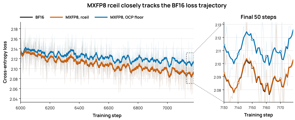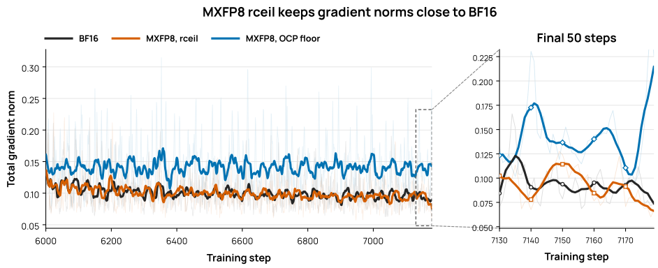Over the final 50 steps, rceil differs from BF16 by +0.00048 mean loss and \(-1.9\%\) mean gradient norm, whereas floor differs by +0.02200 mean loss and +51.1% mean gradient norm.

The direction of this result matches the NVIDIA recipe study: round-ceiling scaling follows the higher-precision baseline, whereas floor scaling produces a visible loss degradation (Mishra et al. 2025).

11.4 The Olmo MXFP8 Recipe for MoE

The optimizer keeps the main weights, the source of truth, in FP32. Forward and dgrad use MXFP8 weight caches. Custom-autograd regions accept and return BF16 at ordinary model boundaries, while selected internal activations and backward gradients remain in MXFP8. Wgrad results accumulate into FP32 gradient buffers; gradient reduction, clipping, and the optimizer update are also performed in high precision. The next forward pass uses caches rebuilt from the updated FP32 main weights, the loop that Figure 55 isolated.

11.4.1 Routed Experts

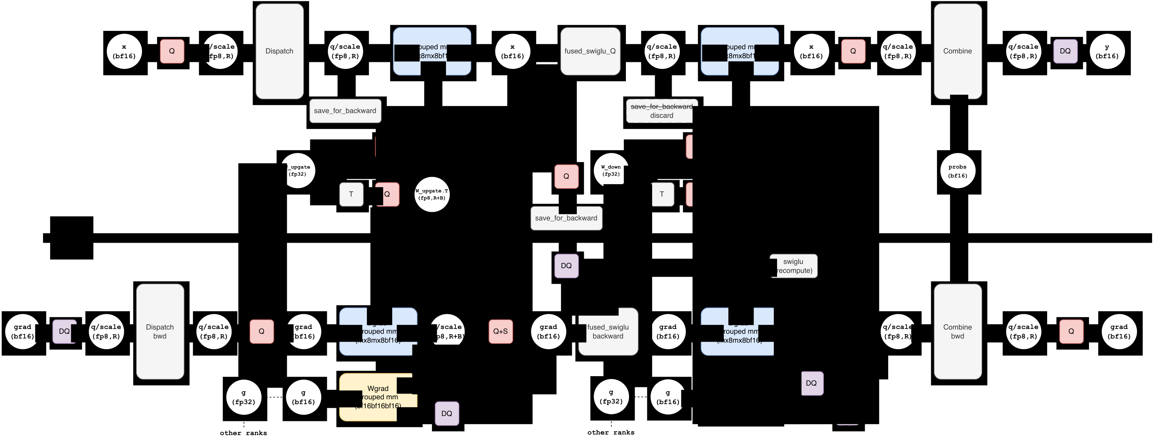
The routed path combines MXFP8 compute with rowwise EP. In forward, the router produces token–expert assignments. Dispatch quantizes each selected BF16 token row into qdata and scales and places those components in the destination expert’s buffers. The up/gate grouped GEMM consumes the dispatched activation and the cached MXFP8 expert weights. A fused SwiGLU-plus-quantization step produces the hidden representation needed by the down projection without requiring a separate BF16-to-MXFP8 pass. The down grouped GEMM then produces a BF16 expert output. That row is quantized for combine transport, and combine reconstructs the route-weighted BF16 token result on the originating rank.

Backward follows the data dependencies in reverse. Combine backward applies the route weights while quantizing the output gradient for transfer to the ranks that hold the selected experts. Dgrad uses the orientation-specific MXFP8 weight caches. Where two adjacent backward stages inside the fused autograd region agree on layout, their qdata and scales pass directly between those stages, avoiding a DQ–Q cycle. Routed Wgrad currently dequantizes the saved operands and uses BF16 grouped matrix multiplication before accumulating the resulting weight gradient into the high-precision sink. Dispatch backward quantizes the input gradient to MXFP8 for transfer and returns it in BF16 to the originating token ranks.

The routed-expert recipe is therefore mixed precision: MXFP8 where scaled GEMM or transport benefits, BF16 at ordinary model interfaces and the current grouped-Wgrad contraction, and FP32 for accumulated gradients, FP32 main weights, and optimizer states.

Figure 57 puts these boundaries into one autograd view. The upper path follows forward execution from dispatch through combine; the lower path follows the corresponding dgrad, Wgrad, and communication work in backward.

Figure 57Interactive · conceptual autograd view, no timing

Where routed values are MXFP8, BF16, or FP32—forward and backward

Highlight

PrecisionSaved · recomputedQ · DQ · TCommunication

Go to stage

1 Dispatch2 Up/gate GEMM3 SwiGLU4 Down GEMM5 Combine

• MXFP8 qdata + scales
• BF16
• FP32
• MXFP8 grouped GEMM
• BF16 grouped GEMM

Dispatch → Combine, left to right in forwardScroll →

View · Precision

“The routed-expert recipe is therefore mixed precision: MXFP8 where scaled GEMM or transport benefits, BF16 at ordinary model interfaces and the current grouped-Wgrad contraction, and FP32 for accumulated gradients, FP32 main weights, and optimizer states.”

Section 11.4.1

Point at, tap, or tab to any value or operation to read its notation.

Conceptual autograd view redrawn from the figure’s source with the same nodes, labels, and arrows; long weight names are drawn as ellipses so they stay legible. On wide screens the drawing is shown whole in two rows, cut between stages 2 and 3; lettered circles A–C join the three arrows that cross the cut (forward continues from row 1 to row 2, backward returns from row 2 to row 1). Stage bands group the figure’s columns for navigation; they are not kernel boundaries.

Figure 57. Routed-expert MXFP8 forward and backward. Forward quantizes routed rows for dispatch, applies MXFP8 grouped GEMMs for the up/gate and down projections, and quantizes the combine payload. Backward reverses the communication path, uses MXFP8 weight caches for dgrad, and uses the current BF16 grouped-GEMM path for Wgrad before accumulation into FP32 gradient buffers that are then reduced with the other ranks’ contributions (dashed arrows). The drawing also identifies saved, discarded, recomputed, quantized, and dequantized values across the custom-autograd boundary. Notation: (fp8, R) is qdata with rowwise scales; (fp8, R+B) keeps rowwise plus blocked (swizzled) scales; Q, DQ, and T are quantize, dequantize, and transpose; Q+S is a fused quantize-plus-swizzle; mx8mx8bf16 and bf16bf16bf16 name each grouped GEMM’s two input dtypes and output dtype. Weight labels treat \(W\) as the right-hand operand (\(xW\)), so \(W\) and \(W\).T correspond to \(W^\top\) and \(W\) in the notation of the text.

11.4.2 Dense and Shared-Expert Linears

The same cache-and-update scheme applies outside the routed experts. Olmo replaces selected attention projections and shared-expert linears with MXFP8Linear. Each weight has forward and dgrad caches derived from its FP32 main weight, and Wgrad is routed to the same high-precision accumulation path used by the DDP optimizer.

The saved-input policy is operator-specific. The packed QKV projection saves its Wgrad input in the MXFP8 RHS layout. The attention output projection keeps its Wgrad input in BF16 because the surrounding attention graph already keeps the relevant BF16 activation alive; adding an MXFP8 copy would not provide the same memory benefit. Attention projections thus use operator-specific compute and saved-activation precision.

Shared experts use the same forward/dgrad cache principle, but their shapes and replica groups follow the shared-expert parameter group rather than the routed-expert group. The recipe evaluated here uses one shared expert with MXFP8-only compute-weight storage, and both shared-expert linears save their Wgrad inputs in MXFP8.

11.4.3 MXFP8 Activation Saving Without MXFP8 Compute

Storage precision and compute precision are independent choices. Olmo’s saved-tensor hooks can pack selected BF16 activations, including the query, key, and value tensors saved for attention backward, into MXFP8 and dequantize them only when backward consumes them. The surrounding forward GEMM does not need to use MXFP8 for this mechanism to reduce saved-activation memory.

Figure 58Interactive · conceptual, nominal bytes per value

Pack it for backward—but only if it replaces a BF16 copy

Saved value

Save BF16MXFP8 replaces itMXFP8 added to a kept BF16 copy

Phase

Whole pathForwardBetween passesBackward

Full-size diagramSwipe →

Retained from forward to backward · nominal bytes per value

• Save BF162baseline
• MXFP8 replaces it33/32−31/32 B per value
• MXFP8 added to a kept BF16 copy2 + 33/32+33/32 B per value

• BF16 · 2 B
• E4M3 qdata · 1 B
• E8M0 scale · 1/32 B

“Replacing a unique BF16 saved tensor with this representation saves 31/32 bytes per value, a nominal reduction of 1 − 33/64 ≈ 48.4%.”

Section 11.1.2

“Olmo’s saved-tensor hooks can pack selected BF16 activations, including the query, key, and value tensors saved for attention backward, into MXFP8 and dequantize them only when backward consumes them.”

Section 11.4.3

“It also trades Q during forward and DQ during backward for lower peak memory.”

Section 11.4.3

Point at, tap, or tab to a part of the diagram to read its notation.

Conceptual diagram from the figure’s source. The lifetime lane and byte bars are web additions using the report’s nominal bytes per value (Equation for B_MXFP8, ignoring blocked-layout padding); they are not measured memory.

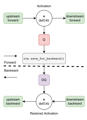
Figure 58. Saving a quantized activation for backward. Forward quantizes the BF16 activation before save_for_backward; backward dequantizes it only when a BF16 consumer needs the value. This saves memory only when the quantized representation replaces, rather than supplements, another retained BF16 copy.

This option is profitable only when the packed tensor replaces a BF16 tensor that would otherwise remain live. It also trades Q during forward and DQ during backward for lower peak memory. Storage-only MXFP8 is therefore a configuration choice separate from MXFP8 compute.

11.4.4 Kernel Problems and Fusions

MXFP8 creates useful fusion opportunities because an intermediate often needs to be transformed before its next consumer. The integrated routed path fuses SwiGLU with row quantization, and combine backward fuses route weighting with gradient quantization. Both avoid writing a large BF16 intermediate solely to read it again for Q. Weight caches similarly move weight quantization from the microbatch path to the post-update boundary.

The current recipe transfers qdata and scales separately. Paired or packed qdata-plus-scale transport and direct weighted-quantize-plus-transfer kernels are prototypes outside the evaluated recipe. For routed Wgrad, global DQ followed by BF16 grouped GEMM was faster than the natural MXFP8 contraction on the measured development shapes, whose reduction dimension and scale layout do not align well with the native block-scaled operation. Table 25 summarizes these choices.

11.5 Throughput Benchmark

We compare four modes to separate the attention-projection contribution from the combined MLP-and-EP contribution: a BF16 reference; MXFP8 for the QKV and output projections in attention; MXFP8 for the dense, shared, and routed MLPs together with MXFP8 rowwise EP transport; and the combined recipe.

Figure 59 reports a controlled four-B300 experiment whose configuration is summarized in Table 26. Throughput is total work divided by wall time over the timed window, which avoids both first-use compilation and an average of already-rounded per-step rates.

Figure 59Interactive · measured, one operating point · four B300 GPUs, EP = 4

Where MXFP8 saved kernel time, and what the end-to-end run gained

Mode

Attention MXFP8MLP + EP MXFP8Combined MXFP8

Kernel view

(a) Sums by family(b) Change vs BF16

(a) What MXFP8 changed on the GPU · rank 0, mean of three captured batches

TargetedDense GEMMGrouped GEMMEP transportNot targetedAttention coreCollectivesOther kernelsAddedQ / swizzle / DQ

▼ marks the GPU-busy union (kernel intervals merged). Family sums overlap across streams and are not an additive wall-time model.

(c) Throughput, three fresh jobs per mode

(d) Peak active memory, same runs

Combined MXFP8 vs the BF16 reference

Throughput+20.6%66.00K vs 54.74K tokens/s/GPU · 1.21×

Peak active memory−8.35 GiB95.05 vs 103.40 GiB · −8.1%

Kernel-duration sum−24.6%1,923 vs 2,551 ms per batch, rank 0

GPU-busy union−20.2%1,855 vs 2,324 ms · kernel intervals merged

Added Q / swizzle / DQ262.1 ms10.3% of the BF16 kernel sum

Plotted from the experiment’s figure metadata and repetition log, the values behind the original figure. Changes by family are computed from the plotted segment sums. Panel (a) uses profiled runs; panels (c) and (d) use unprofiled runs; configuration in Table 26. Systems measurements at one operating point, not training-quality evidence (Section 11.3.5).

Figure 59. Kernel-time breakdown, throughput, and memory across the four MXFP8 modes. The combined recipe reduces the rank-0 kernel-duration sum by a quarter. Panels (a,b) use profiled kernel durations to identify changed work; panel (c) uses unprofiled runs for throughput because tracing perturbs the launch-heavy combined path. (a) Kernel-duration sums per captured train batch on rank 0 by kernel family, means of three captured batches per mode. Teal families are the ones MXFP8 targets, gray families are not targeted, and pink is the added quantization, scale-swizzle, and dequantization work (75.5, 203.1, and 262.1 ms per batch; 3.0%, 8.0%, and 10.3% of the BF16 sum). Family sums overlap across streams and are not an additive wall-time model; the triangle marks the union of kernel-busy intervals, which shrinks by 1.3%, 16.3%, and 20.2%. (b) Change of the three targeted families relative to BF16; the bars in each row are, top to bottom, dense GEMM, grouped GEMM, and EP transport, in the colors of (a). The EP-transport family includes barrier kernels; the payload-moving kernels alone fall by 41% in both the MLP+EP and combined modes, so part of the combined \(-50\%\) is reduced waiting. (c) Throughput change over three fresh distributed jobs per mode; bars are means of the three ten-step windows and dots are the repetitions. The BF16 reference is 54.74K tokens/s/GPU and the largest sample standard deviation is 0.14K, smaller than the dot markers. (d) Peak active memory change in the same runs from the 103.40 GiB BF16 reference. Four B300 GPUs, EP\({}=4\), uniform routing, and identical initialized weights, inputs, and routing in every mode (Table 26); these are systems measurements at one operating point, not training-quality evidence (Section 11.3.5).

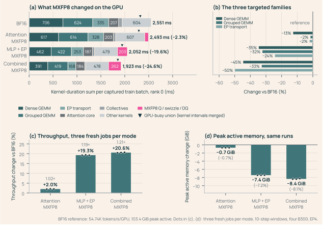
Quantizing attention projections alone gives a modest benefit at this shape: quantization and layout work offset part of the GEMM savings. The MLP and EP path supplies nearly all of the gain. It accelerates the large dense and expert GEMMs and cuts the fixed rowwise EP buffer allocation from 5.00 GiB in BF16 to 2.836 GiB for MXFP8 qdata and scales. Combining both paths gives the highest throughput, about 21% above the BF16 reference, and the lowest peak active memory.

The rank-0 profiles in Figure 59(a,b) support this attribution. The three families MXFP8 targets account for 65% of BF16 kernel time and fall by about a quarter to a half once the MLP path is quantized, while the added conversion work costs a tenth of BF16 kernel time. The untargeted families contribute a much smaller share of the reduction.

These short performance runs verify the systems comparison, not long-horizon training quality. Their first logged loss is identical and their first gradient norms are close under the matched initialization, while the longer continuation experiment in Section 11.3.5 provides the training-trajectory evidence for the selected scale recipe.