
Multiple ungated shared experts can be merged. Several recent MoE designs expose the number of always-active shared experts as a choice; Olmo-core supports at most one ungated shared expert (several shared experts require a learned shared-expert gate), because any larger ungated count expresses the same model class as one wider shared MLP. Suppose every token is sent to several shared experts, every shared expert receives the same input, and their outputs are added without expert-specific, input- or task-dependent gates. The same function can be computed by one shared multilayer perceptron (MLP) whose intermediate width is the sum of their widths (Figure 68). The number of named shared experts is therefore only a partitioning choice; the architectural quantity is the total shared width.
Interactive · conceptual algebra on toy weights, nothing measured
Repartition one set of weights, then try to break the merge
Drag a dashed mark on E star (or focus it and use the arrow keys) to move columns between experts, or choose Ns. Then change the coefficients.
ms = 10 + 8 + 6 = 24 toy columns · parameters 3·d·ms = 432 in both forms · 3 modules or one, same ideal FLOPs
Every coefficient is 1 for every token: the plain sum of Equation 76, one fixed MLP.
Each expert keeps one constant: fold cj into the rows of Wd(j). Still one fixed MLP.
One gate scales the whole branch, a(x)E star(x) (Equation 77). The experts still merge; only the outer gate remains.
The coefficients differ by expert and change with the token, so D(g(x)) is not fixed (Equation 78). Folding Token A’s gj into Wd star reproduces Token A only.
With one shared expert, a per-expert gate g1(x) is itself one branch gate a(x) (Equation 77), so the per-expert case is the one-gate case.
Same weights, two groupings (Equation 75)
Coefficients on each branch
| Token | E1 | E2 | E3 |
|---|---|---|---|
| Token A | 1.00 | 1.00 | 1.00 |
| Token B | 1.00 | 1.00 | 1.00 |
Output y, six toy dimensions
Token Amatch
largest difference 3.0 × 10⁻⁸float32 rounding
Token Bmatch
largest difference 3.0 × 10⁻⁸float32 rounding
- Ns experts, summed
- One shared MLP, fixed weights
- Difference
Toy weights (d = 6, ms = 24 columns, fixed random seed), evaluated in float32 in your browser; for Ns = 3 the widths follow the figure’s drawn proportions (2.2 : 1.6 : 1.2 cm), rounded to whole columns: 10, 8, 6. Conceptual: these are not model weights or measurements. Any nonzero difference in the unit, fixed and one-gate cases is float32 rounding from evaluating the same products and sums in a different order, as the report notes that separate kernels may accumulate floating-point terms in a different order.
Original report figure
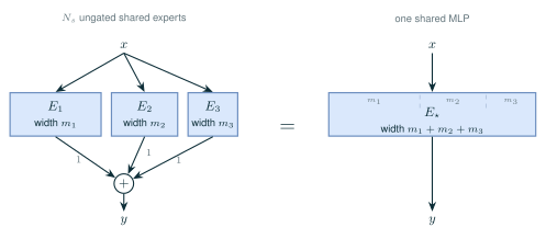
MoEfication uses the same intermediate-dimension partition of a Transformer feed-forward network, and DSMoE writes the equivalence explicitly for a SwiGLU MLP (Zhang et al. 2022; Lv et al. 2025). At fixed total shared width, changing only the number of ungated shared modules does not change the function class.
20.1 The Collapse Is Exact
Let shared expert \(j\) have intermediate width \(m_j\). Using row-vector notation, write its SwiGLU computation as (Shazeer 2020) The gate projection \(W_g^{(j)}\) (part of SwiGLU, not an output gate) and the up projection each have \(m_j\) columns, and the down projection has \(m_j\) rows. Form one wider MLP by concatenating the gate and up projections and stacking the down projections: Because SiLU and the elementwise product act independently along the intermediate dimension, multiplication by the stacked down projection adds the partitions:
The same construction applies to an ordinary two-layer MLP. Fixed expert-specific coefficients do not change the represented function, although they change training dynamics (Section 21): for \(\sum_j c_jE_j(x)\), absorb each constant \(c_j\) into the corresponding rows of \(W_d^{(j)}\). A single input- or task-dependent gate shared by the entire branch also does not require several experts, since \[ a(x)\sum_j E_j(x)=a(x)E_\star(x). \tag{77} \] Among coefficient choices, only distinct input- or task-dependent coefficients \(a_j(x,t)\) generally prevent this fixed reparameterization; the next subsection lists other mechanisms that also preserve expert identity.
The wide and partitioned forms have the same parameters and ideal model FLOPs, and their parameter gradients map slice by slice. When initialization, optimizer settings, and optimizer variables are also mapped in the same way, an element-wise optimizer such as AdamW follows the same training trajectory in both forms; a matrix-wise optimizer such as Muon (Section 4) generally does not, because it updates the wide matrix differently from its slices. Separate kernels may accumulate floating-point terms in a different order, and the two layouts may have different systems performance, but neither effect creates a new represented function.
20.2 Dynamic Gates Preserve Expert Identity
Multiple shared experts become a real architectural choice when the branches are no longer fixed partitions of one MLP. Let \(h_j(x)\) denote expert \(j\)’s intermediate activation of width \(m_j\), and let \(g_j(x,t)\) be its coefficient for input \(x\) and, when applicable, task \(t\). Concatenate the activations as \(H(x)=[h_1(x)\ \cdots\ h_{N_s}(x)]\). The gated merge can then be written as
When the coefficients differ by expert and vary with the input or task, \(D(g(x,t))\) cannot generally be absorbed into the fixed down projection \(W_d^\star\). This is the precise boundary of the collapse. A common scalar \(a(x,t)\) applied to the whole sum does not change this: then \(D=aI\), the experts still collapse into \(E_\star\), and only the outer branch gate remains. Conditional selection, per-expert normalization, different inputs, and branch-specific operations also preserve expert identity.
Earlier MoE architectures illustrate this boundary. One terminology distinction is important: in multi-task learning, a “shared expert” usually means an expert whose parameters are available to several tasks. It does not necessarily mean the always-active shared branch used in recent language-model MoEs. Table 36 therefore lists these models as precedents for separately gated shared experts, not as counterexamples to the ungated equivalence.
| Architecture | Expert structure | Gate and evaluation | Why experts stay distinct |
|---|---|---|---|
| Adaptive local experts (Jacobs et al. 1991) |
Common expert bank; every expert receives the input | Normalized, input-dependent responsibilities for individual experts | Each expert receives a different dynamic coefficient |
| Hierarchical MoE (Jordan and Jacobs 1994) |
Experts organized beneath a tree of gates | Input-dependent coefficients composed along each path | The effective coefficient varies by expert and input |
| Sparsely-gated MoE (Shazeer et al. 2017) |
Globally available feed-forward expert bank | Noisy top-\(K\) routing evaluates and weights a selected subset | Both the coefficients and executed experts vary |
| One-gate Mixture-of-Experts (OMoE) (Ma et al. 2018) |
One expert pool supplies all task towers | One input-dependent vector gate forms a common dense mixture | One gating network still emits one coefficient per expert |
| Multi-gate Mixture-of-Experts (MMoE) (Ma et al. 2018) |
Expert parameters are shared across tasks | Each task has its own input-dependent softmax vector | The same input can expose a different mixture to each task |
| CGC / PLE (Tang et al. 2020) |
Multiple shared experts coexist with task-specific experts | Task gates separately weight both groups; PLE stacks these units | Every shared expert remains separately addressable |
In the one-gate baseline, “one gate” means one network that emits a vector of expert coefficients, not one scalar multiplying the sum. Multi-gate Mixture-of-Experts (MMoE) makes the task dependence explicit, while Customized Gate Control and PLE add separately gated task-specific and shared banks. Dense vector gating and sparse top-\(K\) routing both prevent the collapse for the same algebraic reason; sparsity additionally changes which expert computations execute.
20.3 Expert Count Is Not Shared Width
The equivalence changes how shared-expert designs and ablations should be reported. For an ungated shared branch, the primary parameter-size variable is not \(N_s\) alone. Increasing the number of fixed-width shared experts increases \(m_s\), so it tests additional unconditional parameters and compute rather than an independent benefit from having more expert identities. A count ablation isolates expert partitioning only when total shared width remains fixed; under the assumptions above, such an ablation should differ only through numerical and systems effects.
DeepSeekMoE provides a prominent always-active shared-expert construction (Dai et al. 2024). The collapse is compatible with useful shared parameters, since an unconditional branch may still capture common knowledge; it shows only that several unweighted shared partitions can be represented as one wider branch with the same total parameter size.
20.4 Shared and Routed Widths Are Independent
This result directly motivates Olmo’s representation. Olmo uses one shared MLP and chooses its intermediate width independently from the width of one routed expert. There is no mathematical reason for the two widths to match. The shared width controls the unconditional parameters applied to every token; the routed width controls the parameters contributed by each selected route.
For example, the study configuration analyzed in Section 21 uses routed-expert width 2,560 and shared width 1,280. Calling the latter “half of one routed expert” is only a comparison of widths. It is already the complete shared branch. Splitting it into two width-640 modules and adding their outputs would produce no new model function; combining two width-1,280 modules would simply create one width-2,560 shared MLP in partitioned form.
One wider MLP can also expose a larger GEMM and fewer module launches, but the mathematical identity alone does not predict throughput. Tensor placement, quantization scales, and available kernels can make one physical layout faster than another. Olmo’s use of one shared MLP follows from the functional equivalence, not a measured performance advantage. Its total width remains a model-recipe choice independent of routed-expert width.