
Section 20 established that several ungated shared-expert partitions collapse into one wider shared MLP. After choosing that shared branch, the model recipe must specify how to weight it against the token-dependent routed branches.
An MoE layer may contain both routed experts, selected separately for each token, and a shared expert, evaluated for every token. The routed and shared branches are projected back to the same model width before they are added, but that does not determine how strongly each branch should enter the sum. A normalization that appears innocuous can shrink the MoE output, change its Jacobian, and rescale the gradients of routed and shared parameters by different amounts.
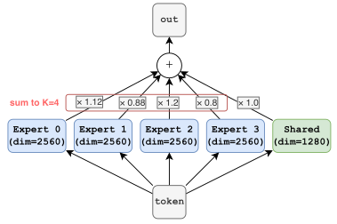
For token \(x\), let \(\mathcal{S}(x)\) contain the \(K\) selected routed experts, let \(f_i(x)\in\mathbb{R}^{d_{\mathrm{model}}}\) be routed expert \(i\)’s output, and let \(g(x)\in\mathbb{R}^{d_{\mathrm{model}}}\) be the shared-expert output. We write the merge as The coefficients \(r_i(x)\) determine the routed contribution, while \(s(x)\) sets the gain of the shared branch (Figure 69). As Appendix E shows, public MoE implementations make substantially different choices for both quantities (DeepSeek-AI et al. 2024; Muennighoff et al. 2024; Yan et al. 2026). We therefore treat the merge rule as part of the model and initialization recipe.
Figure 69Interactive · conceptual coefficients, no measured quantities
Reweight one token’s routed experts: under the Olmo rule the gains still average one
This token’s merge · Equation 80
yMoE = 1.12f0 + 0.88f1 + 1.20f2 + 0.80f3 + 1.00g
- Routed gains
- Σri = 4.00 mean 1.00 per selected expert
- Shared gain
- s = 1.00 every token, no router
Drag a routed gain bar, or focus it and use the arrow keys (or the − / + buttons); the other routed weights rescale so that Σpi stays 1.
- Routed expert gain ri
- Shared expert gain s
- 1 = a dense block’s coefficient
- Width-weighted mean āw
Box widths are proportional to intermediate width (dr = 2560, ds = 1280, the widths of the report’s study); every branch returns a model-width tensor before the addition. Bar heights are merge coefficients, so a bar’s area (width × coefficient) is its term in the width-weighted mean āw (Equation 84); the areas fill the boxes’ total width only when āw = 1. Gains are the figure’s example or weights you set; the variance ratio is Equation 85 evaluated for them, not a measurement.
Original report figure
21.1 A Dense MLP Provides the Scale Reference
A dense SwiGLU MLP provides a useful reference because its intermediate dimension can be partitioned exactly. Split its up, gate, and down-projection weights into \(K\) blocks of width \(d_r\), the routed-expert intermediate width, and one block of width \(d_s\), the total shared width (\(m_s\) in Equation 79). Matrix multiplication distributes across this partition, giving \[ f_{\mathrm{dense}}(x) = \sum_{i=1}^{K} f_i(x) + g(x), \qquad d_{\mathrm{act}}=K d_r+d_s. \tag{81} \] Unit coefficients exactly recover a dense MLP formed by concatenating the active intermediate blocks. For the initialization-scale experiment below, \(K=4\), \(d_r=2560\), and \(d_s=1280\), so the matched dense width is \[ d_{\mathrm{act}}=4\times2560+1280=11{,}520. \tag{82} \]
Routing replaces the four unit routed coefficients with data-dependent route weights. Let \(p_i(x)\) denote the selected router probabilities after L1 normalization, so \(\sum_i p_i(x)=1\). Olmo’s production recipes configure the Olmo-core router to use \[ r_i(x)=Kp_i(x), \qquad s(x)=1. \tag{83} \] The combination weight \(p_{t,e}\) of Equation 1 corresponds to \(r_i\) here, not to \(p_i\). If the selected probabilities are uniform, \(p_i=1/K\) and every active branch again has coefficient one. The routed mixture therefore approaches the exact dense decomposition continuously as the selected probabilities approach a uniform distribution.
This choice also accounts for different expert widths without an additional width multiplier. Define the width-weighted mean coefficient \[ \bar a_w = \frac{d_r\sum_i r_i+d_s s}{K d_r+d_s}. \tag{84} \] Equation 83 gives \(\bar a_w=1\) for any \(d_r\) and \(d_s\). Since the width-weighted mean is already one, a further common factor would rescale the whole MoE output rather than compensate for unequal widths. The narrower shared expert already contributes fewer independently initialized intermediate units, so multiplying its output by a second width fraction would count the same width difference twice under this initialization.
Matching the Coefficients of a Partitioned Dense MLP
Selected router probabilities have mean \(1/K\). Multiplying them by \(K\) makes the mean routed coefficient one, matching the coefficient of each block in an additively partitioned dense MLP. The shared branch then enters the same sum with unit gain.
21.2 Predicting Variance at Initialization
The dense decomposition also yields a simple scale prediction. Assume the randomly initialized branch outputs are centered and approximately independent, and that output variance is proportional to intermediate width under the common initialization. Conditional on the router coefficients, the MoE-to-dense output-variance ratio is \[ R_{\mathrm{var}} \approx \frac{d_r\sum_i r_i^2+d_s s^2}{K d_r+d_s}. \tag{85} \] For the Olmo rule, \[ R_{\mathrm{var}}^{\mathrm{Olmo}} \approx \frac{d_r K^2\sum_i p_i^2+d_s}{K d_r+d_s}. \tag{86} \] Uniform routing gives \(\sum_i p_i^2=1/K\) and hence \(R_{\mathrm{var}}^{\mathrm{Olmo}}=1\). Router concentration increases the ratio according to the concentration term \(\sum_i p_i^2\).
Table 37 contrasts this rule with the three alternatives used in our controlled experiment. All four define valid model parameterizations, but they do not begin at the same forward or backward scale.
| Convention | Coefficients | Immediate effect |
|---|---|---|
| Olmo | \(r_i=Kp_i,\quad s=1\) | Unit-average routed coefficients and a unit-gain shared branch. |
| Routed unit sum | \(r_i=p_i,\quad s=1\) | The routed mixture receives one unit in total, while the shared branch independently receives unit gain. |
| Equal branch mass | \(r_i=\tfrac{1}{2}p_i,\quad s=\tfrac{1}{2}\) | Routed and shared contributions split one unit of coefficient mass. |
| Width-proportional unit sum | \(r_i=\dfrac{K d_r}{d_{\mathrm{act}}}p_i,\quad s=\dfrac{d_s}{d_{\mathrm{act}}}\) | A single unit of coefficient mass is divided in proportion to active intermediate width. |
21.3 The Measured Forward and Backward Scales Agree
We test the prediction in a controlled random-initialization experiment summarized in Figure 70. The forward study uses the layer shape of an earlier Olmo development recipe, not the production recipe: \(d_{\mathrm{model}}=2560\), \(d_r=2560\), \(d_s=1280\), and \(K=4\) experts selected from \(N=48\) router candidates. It instantiates only the four selected experts and evaluates 512 random tokens for each of eight seeds. The dense reference concatenates the same selected and shared weights into an exact width-11,520 SwiGLU MLP, so differences arise from merge coefficients rather than different sampled parameters.
The backward study instantiates all 48 routed experts and gathers each token’s four. To make repeated gradient measurements practical, it scales every dimension down by a factor of ten and raises the initialization standard deviation by \(\sqrt{10}\), which preserves the leading-order projection variances. It uses 1024 tokens for each of twelve seeds and applies the same random upstream gradient to every normalization. We report input gradients with router coefficients both fixed and differentiable, separating the expert-path Jacobian from the additional gradient through the router.
Figure 70Interactive · measured, at random initialization · forward full size, backward scaled surrogate
Which merge rule starts at the dense scale, forward and backward?
(a) Forward output RMS relative to matched dense
(b) Input-gradient RMS relative to matched dense
- router coefficients fixed
- including router gradient
(c) Weight-gradient RMS relative to the Olmo rule
- routed down weight
- shared down weight
(d) Cosine similarity to matched dense output
Olmori = Kpi, s = 1
- (a) Output RMS
- 1.016× dense per-seed 1.014–1.017variance 1.032×; Equation 85 predicts 1.032×
- (b) Input-gradient RMS
- 1.016× · 1.054× per-seed 1.013–1.018 · 1.052–1.057router fixed · including router gradient
- (c) Down-weight gradient RMS
- 1.000× · 1.000× identical in all 12 seedsrouted · shared, relative to Olmo
- (d) Cosine to dense
- 0.984 per-seed 0.983–0.986direction of the merged output
Ranges are the per-seed minimum and maximum: forward panels (a) and (d) over 8 seeds × 512 tokens, backward panels (b) and (c) over 12 seeds × 1,024 tokens.
Plotted from the study’s raw CSV summaries, the values of the original figure. Forward: the full-size initialization configuration (dmodel = 2560, dr = 2560, ds = 1280, N = 48, K = 4), 512 tokens × 8 seeds. Backward: the scaled surrogate (dmodel = 256, dr = 256, ds = 128, all 48 routed experts), 1,024 tokens × 12 seeds. Pick a convention, or hover, tap or focus a bar, to read its values and per-seed range. Random initialization only: no trained-model quality is measured.
Original report figure
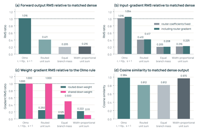
The selected probabilities have \(\mathbb{E}[\sum_i p_i^2]=0.2589\), only slightly above the uniform top-4 value of 0.25. Substituting this measurement into Equation 86 predicts a variance ratio of 1.032, matching the measured value to within 0.03 percentage points. The shared-to-routed branch RMS ratio is \(0.7082\pm0.0028\), close to \(\sqrt{1280/2560}=0.7071\). This confirms that intermediate width already controls branch scale under the tested initialization.
The backward results expose a second advantage of the Olmo parameterization. With router coefficients fixed, its input-Jacobian scale remains close to the dense reference. Its routed and shared down-projection gradients also retain the unit-coefficient scale: the dense reference’s routed and shared down-projection gradient RMS values are \(0.98\times\) and \(1.00\times\) the Olmo values (Figure 70(c) is normalized to Olmo, so it does not plot these ratios). By contrast, routed-unit-sum normalization reduces the routed down-projection gradient RMS to \(0.25\times\) the Olmo value for \(K=4\), while leaving the shared down-projection gradient unchanged. Changing the merge rule is therefore also a parameter-family-specific learning-rate change unless the initialization and optimizer are adjusted with it.
21.4 Scope of the Initialization Result
Olmo’s \(r_i=Kp_i,\ s=1\) rule preserves dense-like forward and expert-path backward scale under the stated architecture, initialization, and approximately uniform selected routing. It has a direct additive interpretation, handles unequal expert widths without a second width penalty, and makes its forward departure from dense scale predictable through \(\sum_i p_i^2\).
The result does not establish a universal MoE normalization. Public models use retained routed mass below one, unit routed mass, learned shared gates, and model-specific routed scales; Appendix E provides a source-pinned comparison. These recipes also differ in initialization, upcycling, router form, and expert width, so their coefficients cannot be ranked in isolation.
Fixed coefficient changes can often be absorbed into expert down projections, but that reparameterization does not make the training recipes identical. It changes initial parameter scale, optimizer states, weight decay, gradient clipping, and effective learning rates. The measurements here characterize random initialization and local backward scale; they do not measure trained language-model quality.