
The remaining sections examine training-recipe choices and a separate benchmarking lesson. We begin with learning-rate scaling and upcycling, turn to operand-value effects in GEMM measurements, then return to shared-expert structure and activation merging. We close with post-training and a comparison with related systems.
Batch-size warmup increases the amount of data processed by each optimizer step as training progresses. It can reduce the number of synchronization and optimizer steps required to process a fixed token budget, but the learning rate must change with the batch. In our batch-size-warmup run, square-root scaling left visible changes in the loss curve at later batch increases.
A common recipe uses the square-root rule (Hoffer et al. 2017), which Malladi et al. (2022) derive for Adam: if the batch grows from \(B\) to \(NB\), then
\[ \eta(NB)=\eta(B)N^{\alpha}, \qquad \alpha=\tfrac{1}{2}. \tag{63} \]
This is the rule used by the batch-size-warmup experiments of Merrill et al. (2025), where the batch grows only after the measured critical batch size has increased. The derivation of Malladi et al. (2022) rests on a stochastic-differential-equation analysis whose same-trajectory condition also scales Adam’s moment coefficients and \(\epsilon\) together with the learning rate. Olmo changes only the learning rate. These results motivate square-root scaling, but do not imply that a single exponent preserves the training trajectory at every batch transition.
16.1 Critical Batch Size Defines the Useful Batch Regime
Let \(g_i\) be the gradient from one training example, \(G=\mathbb{E}[g_i]\) the full gradient, and \(\Sigma=\operatorname{Cov}(g_i)\) the per-example gradient covariance. For a batch of \(B\) independently sampled examples,
\[ \widehat G_B=\frac{1}{B}\sum_{i=1}^{B}g_i, \qquad \mathbb{E}[\widehat G_B]=G, \qquad \operatorname{Cov}(\widehat G_B)=\frac{\Sigma}{B}. \tag{64} \]
Larger batches therefore give less noisy gradient estimates. Under a local quadratic approximation with Hessian \(H\), the expected loss after one stochastic-gradient update is
\[ \mathbb{E}\!\left[L(\theta-\eta\widehat G_B)\right] \approx L(\theta)-\eta\lVert G\rVert^2 +\frac{\eta^2}{2} \left(G^\top H G+\frac{\operatorname{tr}(H\Sigma)}{B}\right). \tag{65} \]
Minimizing Equation 65 gives
\[\begin{aligned} \eta_{\mathrm{opt}}(B) &=\frac{\eta_{\max}}{1+\mathcal{B}_{\mathrm{noise}}/B}, & \eta_{\max} &=\frac{\lVert G\rVert^2}{G^\top H G}, \\ \mathcal{B}_{\mathrm{noise}} &=\frac{\operatorname{tr}(H\Sigma)}{G^\top H G}. \end{aligned} \tag{66}\]
This model predicts two regimes (McCandlish et al. 2018). When \(B\ll\mathcal{B}_{\mathrm{noise}}\), the optimal stochastic gradient descent (SGD) step grows approximately in proportion to \(B\). When \(B\gg\mathcal{B}_{\mathrm{noise}}\), it approaches \(\eta_{\max}\), so enlarging the batch yields diminishing optimization benefit. The often-used simplified noise scale,
\[ \mathcal{B}_{\mathrm{simple}} =\frac{\operatorname{tr}(\Sigma)}{\lVert G\rVert^2}, \tag{67} \]
follows only after removing the Hessian weighting. It is therefore a useful intuition for the turnover, not an exact critical-batch estimator. Large empirical studies likewise find that the useful degree of data parallelism depends on the workload, optimizer, tuning protocol, and target quality (Shallue et al. 2019).
For language-model training, rather than inferring critical batch size from gradient noise, Merrill et al. (2025) branch from a checkpoint and directly find the largest batch whose loss still matches a smaller-batch reference after the same number of tokens. For an Adam branch with batch multiplier \(k\), they set \(B_k=kB\) and \(\eta_k=\sqrt{k}\eta\), measure its smoothed loss \(L_k\) after a fixed token budget, and, with a small loss tolerance \(\varepsilon\), define
\[ k^*=\max\!\left\{k: L_k\leq L_j+\varepsilon\ \text{for every }j<k\right\}, \qquad B^*=k^*B. \tag{68} \]
They find that this empirical critical batch size starts small, grows rapidly, and then plateaus. They also find that the simplified noise scale can underestimate the directly measured value by orders of magnitude and can follow a different trend. Equation 68 tests the useful batch range while taking square-root learning-rate scaling as an input. Critical batch size therefore answers when a larger batch remains token-efficient; it does not determine the exact Adam learning-rate multiplier needed at that transition.
16.2 Adam Does Not Imply One Universal Exponent
Square-Root Scaling Is a Local Approximation
Two independent effects keep the batch exponent from being universal: the optimal step saturates as the batch approaches the turnover scale, and Adam’s slowly adapting second moment lags an abrupt change in gradient noise. The first makes the exponent depend on where the batch sits relative to the turnover; the second can push it above one half at a batch transition. Neither fixes its value.
For learning-rate searches, McCandlish et al. (2018) use a more general saturating curve, which we write as
\[ \eta(B)=\frac{\eta_\infty}{(1+B_{\mathrm{turn}}/B)^{\alpha}}, \tag{69} \]
where \(B_{\mathrm{turn}}\) is the fitted turnover scale and \(\eta_\infty\) is the large-batch limit. These names distinguish this fitted curve from the directly measured \(B^*\) above. Its local log–log slope is
\[ \alpha_{\mathrm{eff}}(B) =\frac{\mathrm{d}\log\eta}{\mathrm{d}\log B} =\alpha\frac{B_{\mathrm{turn}}}{B+B_{\mathrm{turn}}}. \tag{70} \]
The curve behaves like a power law well below the turnover, but its effective exponent decreases toward zero as the batch grows. A fixed power law is thus at best a local approximation, even before accounting for optimizer state.
Adam adds another reason for the exponent to vary. For coordinate \(i\), its update has the form
\[ \Delta\theta_i=-\eta \frac{\mathbb{E}_{\beta_1}[G_i]} {\sqrt{\mathbb{E}_{\beta_2}[G_i^2]}+\epsilon_{\mathrm{Adam}}}. \tag{71} \]
Ignoring the exponential moving averages and \(\epsilon_{\mathrm{Adam}}\) for intuition gives
\[ \Delta\theta_i\approx -\eta\, \frac{\operatorname{sign}(\mathbb{E}[G_i])} {\sqrt{1+s_i/\mathbb{E}[G_i]^2}}, \tag{72} \]
where \(s_i\) is the step-to-step variance of that gradient coordinate. If batch sampling dominates this variance, then \(s_i\propto 1/B\). This motivates square-root scaling for Adam. In practice, however, \(\beta_2\) is commonly close to one, so the second-moment accumulator reacts slowly to an abrupt change in gradient noise. McCandlish et al. (2018) argue that this lag moves the useful exponent from \(0.5\) toward the SGD limit of \(1.0\); their measured Adam and RMSProp exponents lie between these values before the learning rate eventually flattens. This theory supports our suspicion that \(\alpha=0.5\) can slightly under-correct a batch transition, but it does not predict a specific replacement exponent. Their lag argument also assumes \(\beta_2\) near \(0.999\), for which the second moment needs on the order of a thousand steps to react. The run in Figure 66 uses \(\beta_2=0.95\), whose second moment averages over roughly twenty steps, so this lag alone cannot explain a curvature change that stays visible for thousands of steps.
16.3 An Empirical Exponent of 0.53 Smoothed Batch Transitions in Internal Tuning
Figure 66 follows one \(3.21\text{B}@23.10\text{B}\) (active@total parameters) MoE with 24 layers, 48 routed experts, top-\(4\) routing, and one shared expert, trained with AdamW (\(\beta_1=0.9\), \(\beta_2=0.95\)). Its global batch increases through 1, 2, 3, 6, 9, 15, and 24 Mi tokens while the learning rate follows Equation 63. At the later, larger-batch transitions, the smoothed loss shows a visible downward change in curvature. The effect is consistent with the effective learning rate becoming slightly smaller at the transition: multiplying by \(N^{1/2}\) did not fully preserve the local training trajectory.
Figure 66Interactive · measured, one 3.21B@23.10B MoE run · square-root scaling at each batch increase
Step through the batch increases and read the loss on either side
Measured training cross-entropy loss against cumulative tokens, showing the whole run on the report’s 1.80 to 2.20 loss range. Light band: raw loss range per token bucket; dark line: TWEMA; dotted lines: global-batch increases; lower strip: global batch in Mi tokens per step.
Whole run · 7 global-batch stages
1 → 24 Mi tokens per step
Choose a batch increase above, or a row of the table below, to zoom in on it and read its Equation 63 multipliers.
Equation 63 at every batch increase of this run
Plotted from the report’s own series, the 80,000 raw and TWEMA points drawn in the original figure, regrouped for the web into 2B-token buckets for the whole run and 0.25B-token buckets when zoomed. The light band spans each bucket’s lowest to highest raw loss; the dark line is the report’s TWEMA, with no further smoothing. Batch increases and steps are recomputed from the stitched per-step history with the figure script’s rule. Learning-rate multipliers are Equation 63 arithmetic, not logged learning rates: the run used \(\alpha=\tfrac12\) at every increase, and no \(\alpha=0.53\) run is plotted.
Original report figure
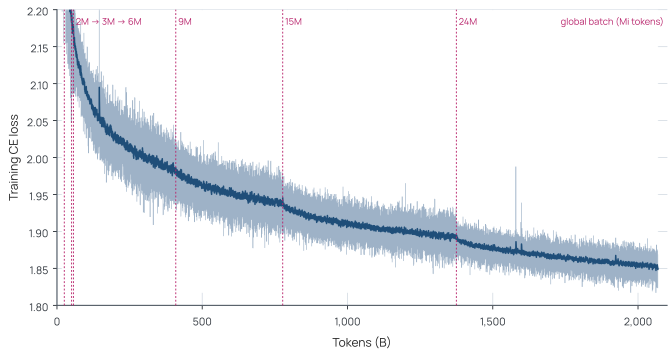
Across repeated internal tuning runs, we found \(\alpha=0.53\) to be a useful empirical setting: it removed the visible change in curvature at the batch increase more consistently than \(\alpha=0.5\). This is a small correction; for a batch doubling, it raises the learning rate only \(2^{0.03}-1\approx2.1\%\) above square-root scaling. Its direction is consistent with the slow-adapting Adam second moment discussed above, but its value was selected from experiments rather than derived from the theory or fitted to the single curve in Figure 66. We therefore present \(0.53\) as an Olmo training recipe, not as a universal scaling exponent.
Section takeaway
Critical batch size identifies when a larger batch remains useful; the Adam learning-rate multiplier still needs tuning. In our internal tuning runs (not plotted here), \(\alpha=0.53\) preserved the local loss trajectory at batch-size transitions more closely than square-root scaling.