
EP reduces routed-expert storage per rank. DDP synchronizes model replicas, but it does not reduce the size of each replica. Without model parallelism, every DDP rank stores all \(N\) routed experts even though each token uses only \(K\). Expert parallelism (EP) distributes the routed-expert pool across the existing DP ranks. Each rank stores its assigned expert shard, and selected token rows move to the ranks that store their experts. This reduces per-rank expert weights and gradient buffers, but adds dispatch and combine communication to every routed layer.
Olmo-core introduces rowwise EP. Conventional all-to-all EP moves tokens in large contiguous blocks, but constructing those blocks requires extra data reordering and can expose dynamic route sizes to the CPU. Rowwise EP keeps routing on the GPU and moves each accepted row directly to its destination, eliminating block packing and the associated host synchronization from Olmo-core’s EP path. NVSHMEM symmetric memory and GPU-initiated communication make this direct placement possible. Section 7 connects it to the underlying network.
5.1 EP Shards Models That Do Not Fit
Persistent training-state memory grows with total parameters.1 Top-\(K\) routing limits how many experts compute for one token, but it does not reduce how many expert weights a rank must store. Without model parallelism, the rank-local model partition is the whole model, so ordinary DDP places all \(N\) routed experts on every one of its \(D\) ranks. Increasing \(N\) can therefore increase total parameter size without increasing active expert work, yet still grow the compute weights and gradient buffers until one replica no longer fits. EP addresses this memory limit by partitioning the routed-expert pool, as in established large-scale MoE systems (Lepikhin et al. 2021; Rajbhandari et al. 2022).
EP uses the existing DP ranks. EP shards expert weights, but it does not require a separate set of ranks in addition to the data-parallel ranks. In the base topology, the same \(D\) ranks that form the dense data-parallel group are organized into an EP_MP rank axis of size \(M_E\) and an EP_DP rank axis of size \(D_E\). Let \(\mathcal{A}_{\mathrm{EP\_MP}}\) and \(\mathcal{A}_{\mathrm{EP\_DP}}\) denote the coordinate sets of these axes. The DP group is their Cartesian product:
\[ \mathcal{G}_{\mathrm{DP}} = \mathcal{A}_{\mathrm{EP\_MP}} \times \mathcal{A}_{\mathrm{EP\_DP}}, \qquad D = M_E D_E. \tag{8} \]
Each pair of coordinates identifies one rank in the DP group. Dense parameters remain replicated across all \(D\) ranks. Routed-expert parameters are sharded across EP_MP and replicated across EP_DP. Equation 8 covers the case without CP. Appendix F derives the folded case, where a CP degree \(C\) gives \(DC=M_E D_E\) within each pipeline stage.
The four-GPU example in Figure 11 shows this rank organization. Begin with \(D=4\) ranks and \(N=16\) routed experts. Set \(M_E=2\) and \(D_E=2\). Each two-rank EP-MP group collectively holds one complete routed-expert set: one rank holds experts 0–7, and the other holds experts 8–15. There are two such EP-MP groups processing different data, so each expert shard has two copies. Attention, the router, and other non-sharded parameters remain replicated across the four dense-DP ranks.
A route connects a token-source rank to an expert rank. The token-source rank holds the token before dispatch and receives its combined contribution. The expert rank stores and executes the selected expert. These are per-route roles, not additional parallel axes.
Figure 11Interactive · conceptual rank layout, no timing
Regroup the same four DP ranks into expert shards
Every layer has this layout (the drawing shows layers 0 and 1). Coordinates are (EP_DP, EP_MP). Hover or tap a token bar under a GPU to follow its route. In the token bars, Left and Right move between expert IDs, Up and Down between GPUs; Enter or Space pins a route.
EP-MP group 0 · with GPU 1
Stores experts 0–7 distributed
EP-MP group 0 · with GPU 0
Stores experts 8–15 distributed
expert 12 runs here
EP-MP group 1 · with GPU 3
Stores experts 0–7 distributed
EP-MP group 1 · with GPU 2
Stores experts 8–15 distributed
Gradient reduction groups
experts over DE = 2 · dense over D = 4
each shard has two copies
Follow a route
A token on GPU 0 that picks expert 12 is dispatched to GPU 1, which stores experts 8–15; combine returns its contribution to GPU 0.
“The token-source rank holds the token before dispatch and receives its combined contribution. The expert rank stores and executes the selected expert.”
Section 5.1
Expert-sharding group (EP_MP)
“Ranks in this group hold different expert shards and exchange routed token rows during dispatch and combine.”
EP Group Definitions box
Conceptual layout transcribed from the original figure: four DP ranks, 16 routed experts, EP-MP = 2 and EP-DP = 2. ME = 1 and ME = 4 apply Equation 8 and Equation 9 to the same four ranks; they are not configurations measured in the report.
Original report figure
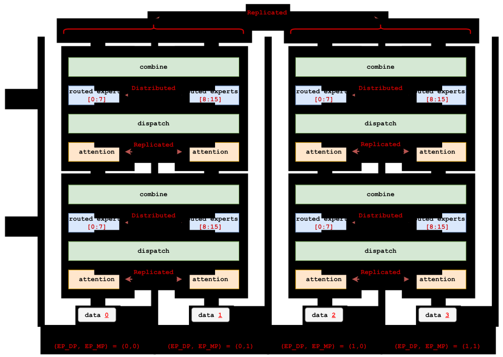
EP Group Definitions
Expert-sharding group (EP_MP). Ranks in this group hold different expert shards and exchange routed token rows during dispatch and combine. Because their expert parameters differ, they do not reduce expert gradients together. |
Expert-replica group (EP_DP). Ranks in this group hold replicas of the same expert shard and reduce that shard’s gradients together. |
EP reduces expert memory and gradient traffic. Figure 9 previewed this decomposition under the report’s BF16-execution and FP32-optimizer policy. Abstracting from that specific precision policy, let \(P_E\) denote the routed-expert parameter count in the complete model. With an even expert assignment, each rank holds approximately
\[ \text{expert weights per rank} \approx \frac{P_E}{M_E}, \qquad \text{expert-gradient elements per rank} \approx \frac{P_E}{M_E}. \tag{9} \]
A rank synchronizes only its local expert shard over \(D_E\) replicas, rather than reducing the full expert pool over all \(D\) ranks. For a fixed EP-DP group size and reduction algorithm, the communicated expert-gradient volume therefore falls with \(P_E/M_E\); the exact network bytes also depend on \(D_E\) and the collective algorithm. Dense, router, shared-expert, and other non-sharded parameters do not receive this EP-MP reduction; they continue to follow the dense DDP group. At fixed expert width, local expert weights and gradient buffers still grow as \(N/M_E\). Keeping these per-rank tensors bounded as \(N\) grows therefore requires increasing \(M_E\).
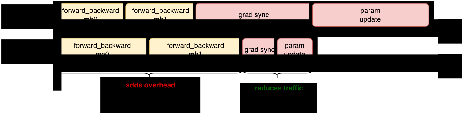
EP can reduce end-to-end step time when parameter-sized work dominates. Dispatch and combine add work to every routed layer and microbatch, whereas gradient synchronization and parameter update occur once per optimizer step. When the gradient-accumulation count is small and the routed-expert state is large, reducing the rank-local expert shard from \(P_E\) to approximately \(P_E/M_E\) can reduce the exposed expert-gradient and update phase enough to outweigh the added per-microbatch EP work. The exact optimizer cost depends on its state placement: optimizer state for the local EP-MP shard may be sharded further over EP-DP. Figure 12 therefore shows a possible operating regime, not a topology-independent speedup.
Figure 12Interactive · conceptual box widths from the drawing, not measured timings
Per-microbatch EP work against a smaller step boundary
- forward_backward
- added EP work (wider box)
- grad sync, param update
Box widths come from the original drawing (forward_backward 120 → 160 units with EP; grad sync and param update 200 → 60 units each) and are illustrative, not measured timings; the forward_backward box repeats once per microbatch. With these widths the lanes cross at seven microbatches: EP ends earlier up to six, the lanes tie at seven, and EP ends later from eight. Whether and where a real run crosses over depends on its measured dispatch/combine and grad sync/param update costs, which the report does not give for this figure.
Original report figure
One single-node eight-B300 run illustrates this operating regime. The run used 32 routed experts, top-4 routing, fixed random routes, eight rank-local microbatches per optimizer step, and 15 measured steps (Table 6).
| Execution path | Tokens/s/GPU | Peak active memory |
|---|---|---|
| No EP | 53,512 | 129.3 GiB |
| Block all-to-all EP8 | 54,063 | 77.85 GiB |
In this run, EP reduced peak active memory by 51.45 GiB at similar throughput. As a single end-to-end feasibility point, it does not show whether reduced expert-gradient synchronization and optimizer-boundary work caused the 1.0% throughput difference, nor does it measure variance or generalize beyond this intra-node configuration. Section 5.3 examines the costs of the block all-to-all implementation used for this comparison.
Per-rank routed activations stay roughly constant as the EP-MP degree grows. Let each rank originate \(T\) tokens before routing. Without EP, the rank processes approximately \(TK\) routed rows. An EP-MP group of size \(M_E\) contains \(M_E T\) source tokens and distributes the resulting \(M_E TK\) routes over \(M_E\) expert ranks. Under balanced routing, each rank therefore still processes approximately \(TK\) routed rows. Increasing \(M_E\) reduces the number of local experts and their persistent training state, but not the average routed rows or capacity-sized communication buffers per rank. Once the local expert shard is small, activations and other execution working memory set a floor, so larger EP-MP degrees provide diminishing peak-memory savings.
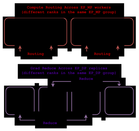
Dense and expert parameters use different reduction groups. A dense gradient must be reduced across all \(D\) dense-DP replicas. An expert gradient must instead be reduced across the \(D_E\) ranks that hold copies of that exact EP-MP shard. Reducing expert gradients across EP-MP would mix different experts; reducing dense gradients only across EP-DP would leave dense replicas out of agreement. The multi-group reducer introduced in Section 4 assigns each gradient bucket to its corresponding replica group.
Figure 13 shows both group types for the four-rank example.
Figure 13Interactive · conceptual rank groups, no timing
Same four ranks, two different group types
EP-DP group 0EP_MP = 0experts 0–7
EP-DP group 1EP_MP = 1experts 8–15
EP-MP group 0EP_DP = 0
EP-MP group 1EP_DP = 1
GPU 0
routed experts [0:7]
attention · router
GPU 1
routed experts [8:15]
attention · router
GPU 2
routed experts [0:7]
attention · router
GPU 3
routed experts [8:15]
attention · router
Rows move inside each EP-MP group
“After the expert pool is sharded, a remote route must dispatch its input row to the expert rank and combine the resulting contribution back at the token-source rank.”
Section 5.1
“This communication occurs in every routed layer and every microbatch, not only once at the global-step boundary.”
Section 5.1
GPU 0 and GPU 1 exchange token rows; GPU 2 and GPU 3 exchange token rows.
The four ranks of the original figure, arranged by their two coordinates: a row is an EP-MP group, a column an EP-DP group, and the whole grid is the dense DP group (the Cartesian product of the two axes). Dots mark token rows or gradients moving inside a group; they are not timings.
Original report figure
EP adds token communication. Before EP, every chosen expert is local to the token-source rank. After the expert pool is sharded, a remote route must dispatch its input row to the expert rank and combine the resulting contribution back at the token-source rank. This communication occurs in every routed layer and every microbatch, not only once at the global-step boundary. The reduced expert memory and gradient traffic therefore come with additional dispatch and combine communication. The next subsection compares these execution paths.
5.2 EP Adds Communication to Dispatch and Combine
MoE dispatches and combines even when every expert is local. A dense MLP applies the same local computation to every token. It has no router, expert-order permutation, or token communication. An MoE layer without EP first chooses experts for each token, permutes the accepted routes into expert-contiguous order, executes the grouped expert MLPs, and then unpermutes and combines the expert outputs. The permutation is local dispatch; the final unpermutation and weighted reduction are local combine. Grouped GEMM requires this expert-contiguous layout even though no rows cross ranks.
EP extends dispatch and combine with an all-to-all exchange. Conventional all-to-all EP extends local dispatch to permute–all-to-all–permute and local combine to unpermute–all-to-all–unpermute. Figure 14 compares this operator path with dense and local-MoE execution. Section 5.3 derives the intermediate layouts and identifies the two additional peer-major/expert-major conversions beyond the local-MoE path.
Figure 14Interactive · conceptual operator order; box widths are not durations
What each path adds around the expert MLP
- layout pass
- rank exchange
- expert MLP
- new in this path
Lanes, box order and relative widths follow the original drawing; widths are not durations. In the block all-to-all lane the three combine boxes are named in the order of Figure 15 and Table 7 (global unpermute, all-to-all, local unpermute); the original drawing labels them local unpermute, all-to-all, global unpermute.
Original report figure
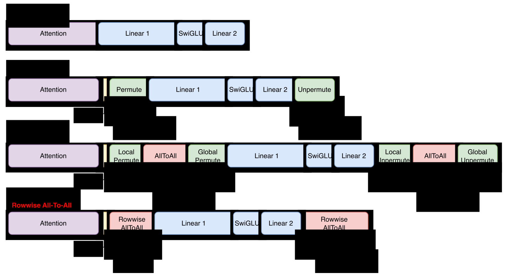
Conventional all-to-all EP adds layout and synchronization work beyond the transfer itself. Relative to local MoE, it adds a rank exchange, up to two additional layout passes, peer-packed buffers, launches, and synchronization around the useful expert GEMMs. These EP-specific costs can remain on the critical path even when network bandwidth is sufficient; Section 5.3 traces them to concrete operations.
Comparing these execution paths fairly requires giving every path the same inputs, routes, and expert work; otherwise a routing or workload difference can be mistaken for an execution-path improvement. The profiled comparison in Section 5.4 matches these factors. End-to-end training speed is a separate question, because EP also changes the gradient-synchronization and optimizer work at the step boundary.
5.3 Packed All-to-All Requires Peer-Contiguous Blocks
Block all-to-all moves one contiguous block per peer. We call the conventional path block all-to-all EP: its transport moves one contiguous block of rows per peer rank, never individual token rows. The path expresses dispatch with PyTorch variable-split all_to_all_single on an NCCL process group (PyTorch Contributors 2026c; NVIDIA 2026n). Each rank supplies one flat send buffer partitioned into a contiguous slice per destination and receives a contiguous slice per source. The call cannot scatter arbitrary token rows directly into arbitrary remote expert slots. The sender must therefore pack all accepted routes for destination rank 0, then destination rank 1, and so on. This peer-block packing is a common expert-parallel implementation pattern (Hwang et al. 2023; Yan et al. 2026). Figure 15 traces the complete packing path for a two-rank example.
Expert order requires a second layout change. After the transfer, the receive buffer is grouped by source rank, not by the local expert that will process each row. A second permutation places those rows into expert-contiguous intervals before grouped GEMM. Combine reverses the layout changes: it converts expert order into source-rank blocks, returns those blocks through the reverse all-to-all, and then restores token order and applies the router weights. The outer token-to-expert and expert-to-token conversions are already present in local MoE. With multiple local experts, packed peer exchange can require two additional peer-major/expert-major conversions, for four passes total; with one local expert, the extra pair is skipped.
Figure 15Interactive · illustrative, the report’s two-rank example · layout and movement, not timing
Follow every row through block all-to-all EP
Route · stage 1 of 10
The router picks two experts per token
Each token gets two expert indices and two router weights (top-2), exactly as in the drawing. Experts 0 and 1 live on rank 0, experts 2 and 3 on rank 1.
- 0/4explicit layout passes
- 0/2rank exchanges (all-to-all)
- not yethost split list
- —route dropped at capacity
Select a token, or a row, to follow its two routes. Arrow keys move between tokens.
Rows, router indices, weights, buffer orders, the capacity formula and the dropped route (E→1) are transcribed from the original drawing. Stages follow its labels and the phases of Table 7. Arrows show rows crossing ranks; positions show data layout and movement, not timing.
Original report figure
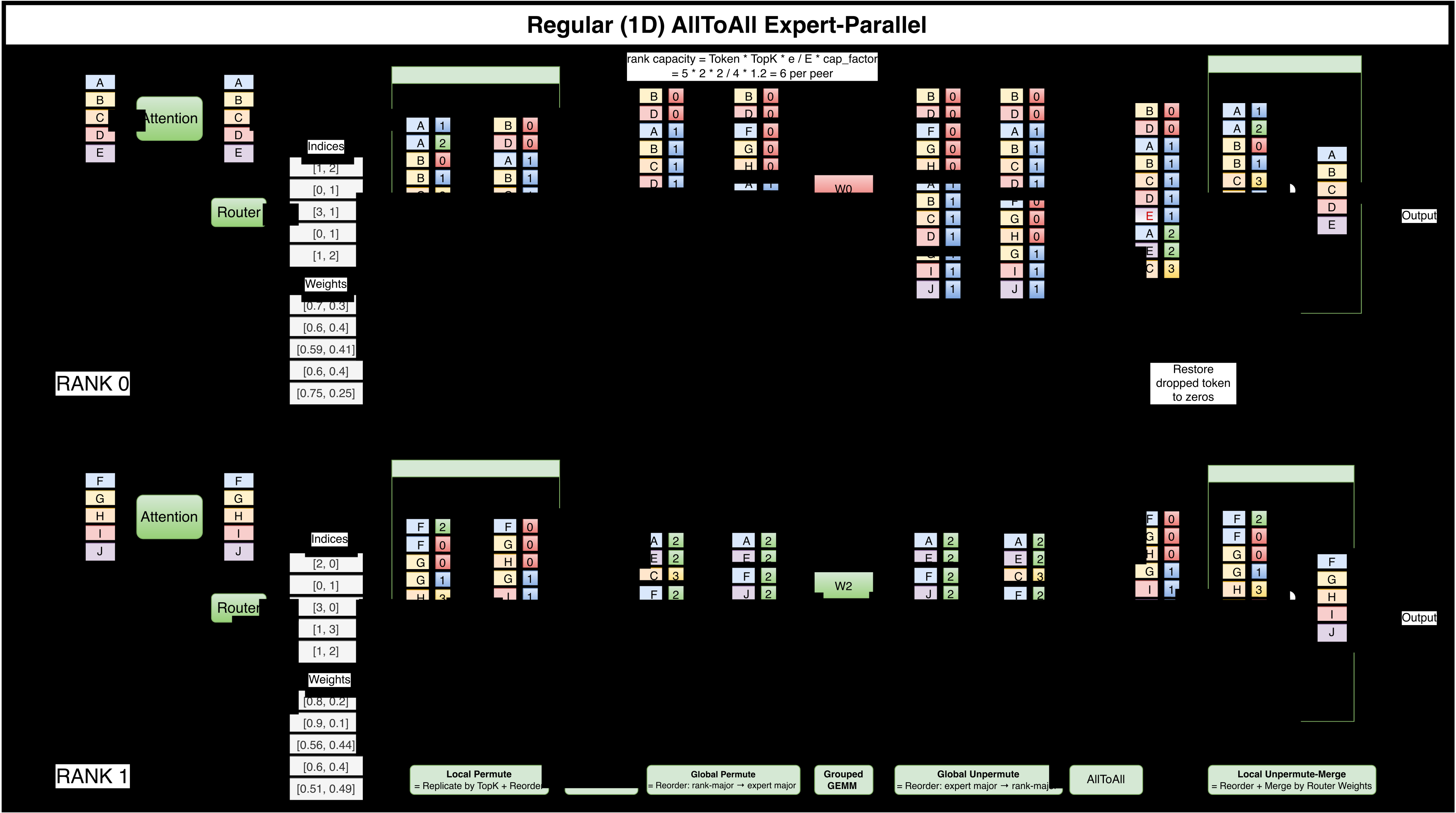
Dynamic peer-block lengths create a host dependency in the current path. Because routing changes the peer-block lengths every microbatch, Olmo-core’s implementation converts GPU-produced peer counts into host split lists before launching the variable-split exchange; when we emphasize this host dependency, we call it the synchronized path. Section 8.4 explains how this device-to-host dependency reduces submission headroom and how independent work can cover, but not remove, the wait.
Faster links shrink only the all-to-all itself. The peer/expert layout conversions, peer-packed buffers, and this implementation’s host dependency remain. Network bandwidth alone therefore cannot explain the cost of the complete block all-to-all path.
5.4 Rowwise EP Removes Block Packing
Rowwise EP transfers each row directly to its expert slot. Rowwise EP replaces block packing with direct row placement: each accepted token row is transferred on its own, straight into the destination buffer row where its selected expert expects it. For \(T\) local tokens and top-\(K\) routing, Olmo-core constructs two GPU tensors of shape \([T,K]\). One gives the destination EP-MP rank for each accepted route; the other gives the row in that rank’s expert-capacity buffer. Negative entries represent invalid or capacity-dropped routes; Section 10.3 defines the capacity policy and its drop metrics, and in stable training the routing distribution stays nearly dropless. A dispatch kernel uses these two indices to move \(x_t\) directly to its destination row. The communication output is already expert-contiguous on each destination rank, so grouped expert computation does not require a packed peer buffer or a second permutation.
The destination row is deterministic. The route-map builder combines the destination expert, the number of earlier accepted routes for that expert, and the offsets of the preceding local experts. It also applies the capacity decision before communication. The map therefore records both the remote destination rank and the precise row consumed by the selected expert. Route counts and overflow metadata remain on the GPU; they are not converted into host split lists for the data movement. Direct placement presupposes that a kernel on the token-source rank can write a row that lives on the expert rank. Section 5.5 introduces the symmetric-memory and GPU-initiated communication (NVSHMEM/RDMA) mechanisms that make remote rows addressable.
Rowwise EP adds indexing and ordering costs. Rowwise movement replaces a small number of block transfers with many indexed row transfers and adds route-map construction, fixed-capacity storage, and explicit write-ordering between communication and compute. It is beneficial only when those costs are lower than the permutations, temporary buffers, and host stalls of the block all-to-all path. Its end-to-end advantage depends on expert shape, EP degree, route imbalance, and network topology, which the current measurements only partly cover.
Figures 15 and 16 make the layout difference explicit. The block all-to-all path packs accepted routes into contiguous destination-rank blocks, exchanges those blocks, and then reorders the received rows into local-expert order. Combine reverses both layout conversions. Rowwise EP instead uses the GPU route map to place each accepted row directly in its destination expert-capacity slot and reverses that indexed movement during combine. It removes packed peer buffers and up to four explicit layout conversions; it does not remove routing, communication, grouped expert computation, or the synchronization that orders remote writes between ranks.
Figure 16Interactive · illustrative, the report’s two-rank example · layout and movement, not timing
Follow every row through rowwise EP
Rows derived from the drawing’s storage order: row = offset of the expert on its rank + earlier accepted routes for that expert (for example B→1: 5 + 1 = 6).
Dispatch · stage 2 of 6
Route-map build: a destination rank and row for every route
“One gives the destination EP-MP rank for each accepted route; the other gives the row in that rank’s expert-capacity buffer. Negative entries represent invalid or capacity-dropped routes…”
Section 5.4
“The route-map builder combines the destination expert, the number of earlier accepted routes for that expert, and the offsets of the preceding local experts. It also applies the capacity decision before communication.”
Section 5.4
- 0 · block: 4explicit layout passes
- 0/2indexed row exchanges
- nohost split list
- E→1route dropped at capacity
Select a token, or a row, to follow its two routes. Arrow keys move between tokens.
Router output, storage order and the capacity formula are transcribed from the original drawing; it stores every route except E→1. Route-map rows are derived from that storage order. Arrows show rows crossing ranks; positions show data layout and movement, not timing. Compare Figure 15 for the block path.
Original report figure
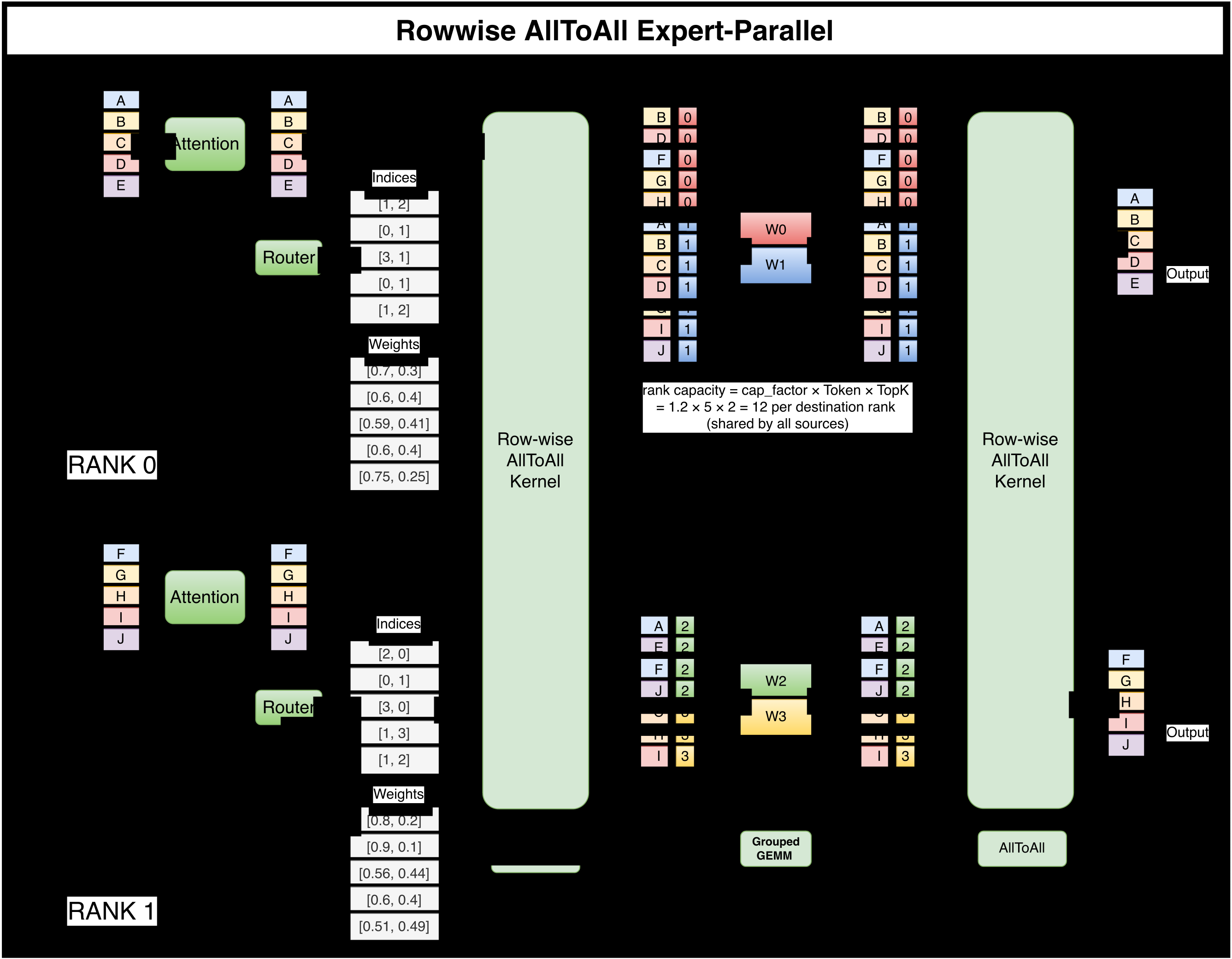
Table 7 groups the displayed ranges from one inspected rank-0 MoE forward instance in each of two configuration-matched traces, each captured on one node with eight B300 GPUs. Both use an eight-layer BF16 model with 128 routed experts, top-8 routing, no shared expert, EP8, and four sequences per rank microbatch. The traces were captured on different nodes, so the comparison is mechanism evidence rather than a controlled performance result.
| Phase | Block all-to-all EP | Rowwise EP | ||
| Operation | ms | ms | Operation | |
| Dispatch | Local permute | 0.351 | 2.298 | Route-map build + row dispatch |
| All-to-all | 1.960 | |||
| Global permute | 0.532 | |||
| Compute | Grouped GEMM | 3.630 | ||
| Combine | Global unpermute | 0.712 | 2.423 | Row gather + weighted reduce |
| All-to-all | 1.970 | |||
| Local unpermute + merge | 0.391 | |||
| Dispatch + combine | 5.916 | 4.721 | ||
Figure 17 shows the same example as two cumulative-duration paths: three explicit block-path stages on each side of expert computation versus one aggregated rowwise phase.
Figure 17Interactive · measured, one profiled forward per path · Nsight Systems traces
Three explicit stages on each side, or one rowwise phase
- Layout transform
- Peer-block collective
- Rowwise phase
- Expert computation
Point at, tap, or tab to a stage to read its duration and see what it corresponds to in the other path.
Durations from the report’s figure script, identical to Table 7. Shares, phase sums and the Δ between the two totals are computed here from those values; both lanes share one axis of cumulative displayed duration, not a clock.
Original report figure
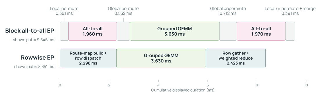
This example is consistent with the intended mechanism: rowwise replaces four explicit layout transformations and two peer-block collectives with a GPU-resident route map and indexed row movement, with device route-map construction included in the rowwise total. The displayed ranges exclude the block path’s host split-list wait (Section 8.4). This instance identifies the affected operations but does not establish the size of the saving across workloads and networks.
Direct placement also lets communication use the MXFP8 representation consumed by grouped GEMM. Olmo can quantize rows during dispatch, let expert grouped GEMM consume the received qdata (quantized data) and scales directly, and return quantized outputs before local reduction. Communication and expert compute thus share one representation without an intervening BF16 materialization. Section 11.4 follows the integrated forward and backward path.
5.5 Symmetric Memory Addresses Remote Rows
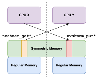
Direct placement requires a remote address. Ordinary device pointers name local memory. Symmetric memory gives the participating ranks corresponding regions in a symmetric heap, so a local offset together with a peer-rank index names the matching remote location (Figure 18). In the current Olmo-core setup, each EP-MP process group forms the NVSHMEM bootstrap world used by its rowwise kernels. All ranks in that group allocate the same set of buffers, with matching shapes and allocation order (NVIDIA 2026s).
Olmo-core uses NVSHMEM because it permits GPU-initiated one-sided operations. A CUDA kernel can issue a PUT to a remote expert row or a GET from one without first constructing a host-managed peer block. This does not mean that NVSHMEM is universally faster than NCCL. It provides the addressability and fine-grained movement required by this particular rowwise design (NVIDIA 2026s, 2026r).
Safe buffer reuse is a separate problem from addressability. A symmetric pointer may remain valid while the value at that address is still needed by an earlier microbatch. Every rank must agree on buffer capacity and initialization before communication begins, and the runtime must prevent a later operation from overwriting a row until its final forward or backward consumer has completed. Matching allocations alone cannot prevent premature reuse; the runtime also needs explicit ordering and buffer-reuse rules.
Figure 18Interactive · conceptual structure, illustrative group of four EP-MP ranks
One offset plus one peer rank names a remote row
Symmetric heap · one-sided PUT
local offset 5 + peer rank 2 → offset 5 in rank 2’s symmetric heap (combine buffer)
Every rank in the group allocated the same buffers in the same order, so offset 5 names the matching location on each of them. Rank 0’s kernel writes the row directly; no host-managed peer block is built first.
The four ranks, eight offsets and two buffer names are illustrative. Tap a row to pick a peer rank and an offset. Buffer reuse across blocks and microbatches: Figure 21 and Figure 22.
Original report figure
5.6 Routes Use PUT and GET
MoE operations and transport directions are distinct. Dispatch and combine describe the MoE computation; PUT and GET describe the direction of the one-sided transfer. Table 8 shows the mapping used by the rowwise path.
| MoE operation | Transfer | Row movement |
|---|---|---|
| Dispatch forward | PUT |
The token-source rank pushes \(x_t\) to the capacity row assigned to the selected expert. |
| Combine forward | GET |
The token-source rank pulls the selected expert outputs and performs the router-weighted reduction locally. |
| Combine backward | PUT |
The token-source rank pushes each router-weighted output gradient to the corresponding expert-output gradient row. |
| Dispatch backward | GET |
The token-source rank pulls the route gradients and sums them into the gradient of the original token row. |
Fan-out favors source-initiated PUT. A top-\(K\) token row may need to reach several expert ranks. With PUT, the token-source rank reads its local row and writes each route into a distinct remote capacity slot. Expressing the same fan-out as destination-initiated GETs makes several peers read the same remote source row, concentrating access pressure at that source (Figure 19).
Figure 19Interactive · conceptual, illustrative ranks and slots, no timing
Where does a top-K fan-out concentrate access?
Rank counts and slot positions are illustrative. Arrows point from the rank that issues the one-sided operation toward the remote address. The dots on the token row count its reads: local under PUT, remote under GET.
Original report figure
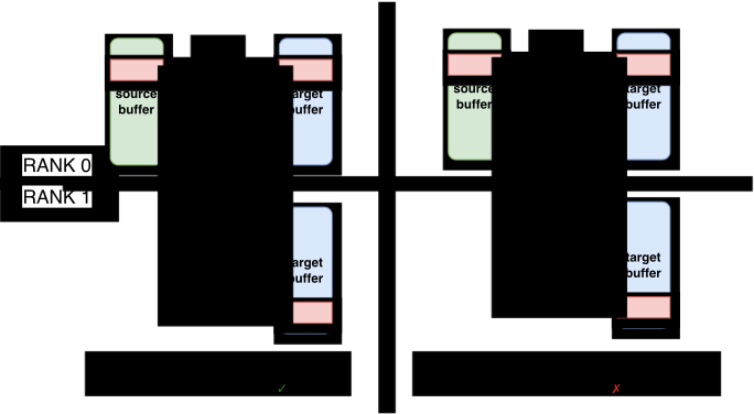
Forward dispatch writes directly into expert-contiguous capacity storage. The expert rank then runs grouped expert computation over the valid row intervals. Forward combine gathers the \(K\) selected expert rows for each local token, multiplies them by their router weights, and sums them into token order. The custom autograd functions save the route map so backward applies the exact transpose movements in Table 8. The router-weight gradient uses the gathered expert outputs and the token-output gradient from the same accepted routes.
Invalid routes remain explicit throughout this path. Rowwise PUT kernels skip negative destinations; combine gathers zero for invalid entries before the local reduction. Capacity handling is therefore part of the route map rather than an implicit property of unwritten memory.
5.7 Buffer Reuse and Ordering Are Explicit in Rowwise EP
A microbatch fills only a prefix of each capacity buffer. Rowwise communication reserves capacity-sized destination buffers, but a microbatch usually writes only a dense prefix of each buffer: the local experts’ rows are packed back to back from row 0, and one unwritten tail follows the last expert. Tail rows may contain values from an earlier use. Expert forward and backward therefore receive the real per-expert row offsets, and grouped GEMM and the expert weight-gradient GEMM (Wgrad) skip the unwritten tail. Clearing the whole capacity buffer is useful as a diagnostic, but it adds unnecessary memory traffic to the normal path.
Direct access avoids staging copies but extends buffer use into backward. Grouped GEMM reads the symmetric dispatch buffer in place instead of copying its contents into a regular tensor. Its saved Wgrad input therefore remains in the same buffer that a later dispatch could overwrite. Figure 20 shows where direct access removes copies; the resulting buffer-reuse constraints depend on how long each consumer needs the data.
Figure 20Interactive · conceptual structure, no measured quantities
Remove the copies on both sides of the symmetric boundary
2 copies across the boundary
One generic producer, transfer and consumer stand for both directions. In (b) the rowwise kernels write and read symmetric memory themselves, removing the staging copies where kernels can target symmetric memory directly; pick a case above to see which parts it names.
Original report figure
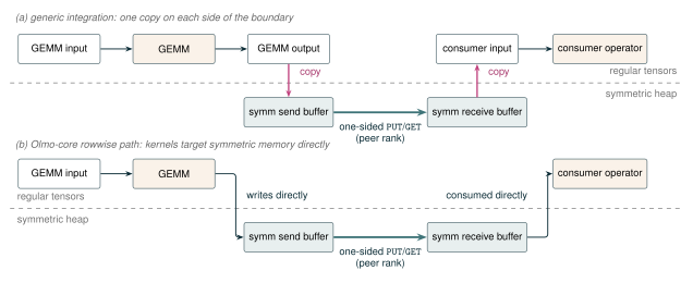
PUT kernel. Conceptual illustration with no measured quantities.Reusing buffers across blocks saves memory but can overwrite saved payloads. Symmetric buffers are allocated collectively and stay resident, so giving every MoE block private symmetric buffers makes resident symmetric memory grow with the number of local blocks. Sharing buffers across blocks removes that growth, but forward and backward visit blocks in opposite orders: block \(\ell{+}1\)’s dispatch would overwrite the payload that block \(\ell\) saved, long before block \(\ell\)’s backward reads it (Figure 21). Whether a buffer faces this hazard is decided by its immediate consumer. The dispatch buffer feeds the up-projection grouped GEMM, which saves its input for Wgrad, so the buffer must survive until backward. The expert-output buffer is only read by the combine transfer, and backward re-routes gradients with the saved route map (the router-weight gradient uses a separate gather capture on the token-source rank), so it is scratch and may be reused as soon as the transfer completes.
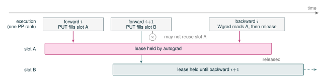
Autograd determines when a buffer may be reused. Under pipeline parallelism, several later forwards may execute before the Wgrad that reads a block’s saved dispatch payload. Remote writes through custom communication kernels are not protected by PyTorch’s ordinary tensor version checks, so Olmo-core attaches autograd-held leases to symmetric payloads that remain visible to backward. Each lease prevents reuse until the corresponding autograd node releases it after its final consumer. When activation checkpointing recomputes the payload for backward, the original forward can instead use shared scratch storage. Figure 22 shows how a lease keeps a dispatched payload available for its backward consumer.
Figure 21Interactive · conceptual step order, no timing or measured quantities
Share one symmetric buffer across blocks, and watch backward
Backward, block 1: Wgrad reads the shared buffer but finds block 3’s payload; block 1’s was overwritten. ✗
Three local MoE blocks, in step order only. “Saved for Wgrad” is the dispatch buffer that grouped GEMM keeps for backward; “Scratch” is the expert-output buffer, read only by the combine transfer; “Recomputed” is the dispatch payload under activation recompute. Drag along the steps or use the arrow keys.
Original report figure
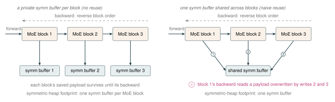
Figure 22Interactive · conceptual event order on one pipeline rank, no timing
Keep the saved dispatch slot until its Wgrad has run
Forward i+1: slot A is leased, so it may not be reused; forward i+1 acquires slot B from the pool.
- slot A leased by forward i
- slot B leased by forward i+1
One pipeline-parallel rank, in event order only. “No lease” shows the hazard the lease prevents; it is not an Olmo-core mode. Two slots and two microbatches are illustrative: under pipeline parallelism several later forwards may run before the Wgrad that reads a saved payload.
Original report figure
One-sided communication requires explicit ordering. Expert compute must not read a destination row before all required dispatch writes are visible. A buffer must not be overwritten while a peer is still reading it, and all ranks participating in a barrier or collective kernel must enter a compatible operation order. The rowwise path uses stream ordering and NVSHMEM completion operations around these phase boundaries. Removing the host split-size wait does not remove distributed synchronization; it moves the required agreement and completion into the GPU execution path (NVIDIA 2026r).
MXFP8 adds a reuse constraint between quantized activations and gradients. As on the BF16 path, Wgrad needs the dispatched input. A BF16 route carries one row; an MXFP8 route carries qdata and scale rows that follow the same destination indices and validity mask. Backward must consume both saved components before the slot is reused for quantized gradient rows. This shared-buffer constraint is one reason Olmo-core fuses dispatch, expert computation, and combine into a single autograd node on the MXFP8 path (Section 11.4).
5.8 DeepEP v2 Provides an Optional EP Backend
DeepEP v2 is an effective inter-node alternative. Olmo-core can select DeepEP v2 for dispatch and combine while retaining its router, capacity policy, expert kernels, autograd integration, and optimizer (Zhao, Zhou, et al. 2025). DeepEP v2 is block-oriented like the path in Section 5.3: it exchanges per-peer batches of rows rather than individual rows. The difference is that packing, transfer, and unpacking happen inside its dispatch and combine calls with GPU-resident metadata, so the model-facing path keeps no host split lists.
Block transfers reduce the NIC request rate. The block orientation matters most across nodes. Within a node, NVLink transfer time is governed mainly by payload bytes, so rowwise EP’s many small row transfers cost little beyond the bytes they move. Across nodes, every transfer becomes a request that the network interface controller (NIC) must process, and a pattern that issues one request per route can saturate the NIC’s message rate before it saturates link bandwidth (Section 7 describes the GPU-to-NIC submission path). Aggregating rows into a few large per-peer transfers keeps the request count low. Our observations are consistent with this reasoning, though we have not measured the attribution. DeepEP v2 has performed well in our current inter-node experiments, which makes it useful when an EP-MP group spans nodes (on our eight-GPU nodes, EP-MP degrees greater than eight); rowwise EP remains the production intra-node path.
The trade-off is integration depth. Olmo-core does not control DeepEP’s dispatch/combine kernels and public interface, so it cannot specialize every communication boundary as freely as it can in the rowwise backend. In the current MXFP8 integration (Section 11), forward dispatch transports E4M3 data with E8M0 scales and the expert GEMMs use MXFP8. Forward combine, cached backward dispatch, and backward combine remain BF16. Extending MXFP8 across those remaining communication legs would require new DeepEP kernels and interfaces, not only an Olmo-core configuration change. We therefore use DeepEP v2 as an inter-node option and rowwise EP where its closer integration with Olmo-core’s communication, precision, and autograd implementation is useful.
5.9 Overlap Is Not Free: Resource Contention
A wave schedule splits a microbatch’s routed work into waves and attempts to dispatch wave \(i+1\) and combine wave \(i-1\) while the experts compute wave \(i\). The idea comes from DeepSeek’s inference systems, where Mega MoE in DeepGEMM fuses EP dispatch, the expert MLP, and EP combine into one persistent megakernel that overlaps communication with tensor-core computation (DeepSeek-AI et al. 2026; Zhao, Xu, et al. 2025). We adopted the schedule for training but not the megakernel: the Olmo-core wave path launches ordinary dispatch, grouped-GEMM, and combine kernels on separate streams, so the overlapped stages compete for the same GPU resources instead of sharing one kernel’s internal schedule. Section 15.4 describes MegaMoE, our own BF16 megakernel prototype in the style of DeepGEMM’s Mega MoE, and why we removed it. Wave execution can hide exposed communication, but it also turns one large expert batch into several smaller grouped GEMMs. A complete comparison needs three schedules: no-wave phase-sequential execution, wave-sequential execution, and wave-overlapped execution. Wave-sequential execution is the control that separates the cost of smaller GEMMs from the cost of concurrent kernels. Our archived experiments lack it, so they show whether the complete wave schedule was faster but cannot split the difference between the two causes.
Let \(T_{\mathrm{comm}}\) and \(T_{\mathrm{gemm}}\) be the standalone times for communication and expert computation. Sequential execution costs \(T_{\mathrm{comm}}+T_{\mathrm{gemm}}\). After overlap, the same operations may stretch to \(\widetilde{T}_{\mathrm{comm}}\) and \(\widetilde{T}_{\mathrm{gemm}}\) as they contend for GPU and communication resources, so the overlapped schedule takes \(T_{\mathrm{overlap}} \ge \max(\widetilde{T}_{\mathrm{comm}}, \widetilde{T}_{\mathrm{gemm}})\). Overlap improves elapsed time only if
\[ T_{\mathrm{overlap}} < T_{\mathrm{comm}} + T_{\mathrm{gemm}}. \tag{10} \]
Figure 23 makes the no-wave and wave-overlapped order concrete with one measured forward instance at a 32-SM communication budget; the missing wave-sequential control cannot be inferred from it.
Figure 23Interactive · measured, one rank and one iteration · two-node DeepEP v2, EP-MP = 16, 32-SM budget
Overlap runs communication beside compute, and the forward path still grows
- Dispatch + copy epilogue
- Expert MLP
- Combine + reduce epilogue
- Merge
- Beyond the no-wave end
At 20.0 ms after the first dispatch
- No waveCommunication stream: idleExpert compute: E · Expert MLP
- Four wavesCommunication stream: C0 · Hybrid combineCompute stream: E1 · Expert MLP
Every interval is a row of the report’s timeline table. Percentages and the per-wave sums are computed here from those rows.
Original report figure
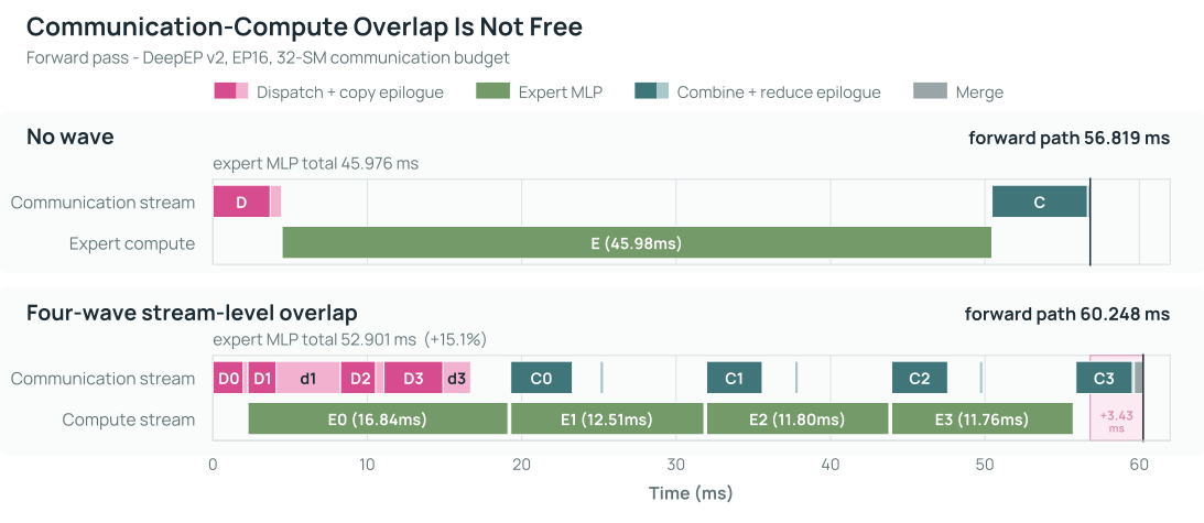
Expert computation takes longer in the wave trace. Figure 23 shows real communication–compute concurrency, yet the displayed wave forward interval is 3.429 ms longer and its expert-compute intervals grow by 15.1% in aggregate. Across the full profiles, the three dominant grouped-GEMM kernel families accumulated 4.63 s in the no-wave trace and 5.74 s in the wave trace. The wave schedule both split the expert work into four smaller grouped GEMMs and ran DeepEP kernels beside them, so these profiles cannot assign the additional time uniquely to GEMM granularity or concurrent resource contention.
Concurrent rowwise communication slows expert GEMM. In a separate two-node, 16-GPU diagnostic with EP-MP\({}=16\), 16,384 tokens per rank, top-\(8\) routing, and \(d=h=6{,}144\), we launched either a rowwise NVSHMEM dispatch or combine transfer concurrently with one grouped expert workload while sweeping the communication launch width from 1 to 128 blocks. Table 9 reports the GEMM stretch and the makespan, the total elapsed time of the concurrent pair. Concurrent communication slowed the grouped GEMM by roughly a quarter at every launch width, and shrinking the communication launch to a single block did not avoid the GEMM slowdown; it stretched communication by an order of magnitude.
| Concurrent pair | GEMM time (ms) | GEMM slowdown |
|---|---|---|
| Grouped GEMM alone | 4.645–4.679 | — |
| GEMM + rowwise dispatch | 5.736–5.874 | 22.9–26.0% |
| GEMM + rowwise combine | 5.724–5.907 | 23.0–27.0% |
| Pair schedule (128-block launch) | Makespan (ms) | |
| Dispatch then GEMM, sequential | 7.768 | |
| Dispatch and GEMM, overlapped | 5.833 | |
| Combine then GEMM, sequential | 7.560 | |
| Combine and GEMM, overlapped | 5.868 |
GEMM stretch alone, however, does not decide the outcome. At the 128-block launch, overlap still shortened the pair’s makespan by 22–25% relative to sequential execution: the wide launch finished communication soon enough to hide behind useful work despite the contention tax, while the one-block launch did not.
The complete wave candidate did not beat its no-wave baseline. A two-node DeepEP v2 sweep measured BF16 forward and backward for EP-MP\({}=16\), 128 experts, top-\(8\), 16,384 tokens per rank, and \(d=h=8{,}192\). The four-wave path used an expert-major static layout and overlapped dispatch, expert compute, and combine. Figure 24a shows that it remained slower than no-wave execution at every matched communication-SM setting.
Figure 24Interactive · measured, standalone DeepEP v2 benchmarks · max-rank medians
Tune the communication-SM budget, then compare against the best no-wave point
(a) Two nodes: complete forward + backward
EP16, 128 experts; expert-major layout
No wave wins every budget; best at 32 SMs
- No wave
- Wave overlap
Best: no wave at 32 SMs, 155.014 ms. Wave overlap is slower at every budget.
(b) Different four-node configuration
EP32, 256 experts; passes timed separately
Wave wins at 8; no-wave 32 is best overall
- No wave
- Wave overlap
- Forward
- Backward
Best: no wave at 32 SMs, forward 11.570 ms and backward 19.768 ms. Wave overlap wins only at 8 SMs.
DeepEP communication SM budget · panels use independent vertical scales; lower is better
Plotted from the report’s sweep table, which the report plots as absolute times. The percentage view is computed here as wave ÷ no wave − 1 (the formula defined in the report’s figure generator). One archived run per point; no wave-sequential control.
Original report figure
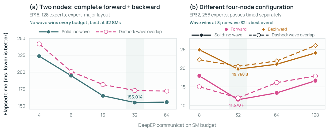
The sweep also shows why lowering the communication SM count is not sufficient: at four and six SMs communication became the bottleneck, while larger budgets still did not recover the no-wave time.
Overlap helps at eight SMs, but no-wave at 32 SMs is faster. A later four-node, 32-GPU source-token-major experiment is shown in Figure 24b. At the eight-SM budget, where communication dominates, four-wave execution beat no-wave for both forward and backward. At 32 SMs, no-wave was faster again and was the best measured point for both passes. Overlap can therefore help a communication-constrained configuration without improving the best configuration of the sweep.
DeepSeek-V3, Megatron-Core, DeepEP, COMET, and Lancet report overlap designs that win in their settings (DeepSeek-AI et al. 2024; Yan et al. 2026; Zhao, Zhou, et al. 2025; Zhang et al. 2025; C. Jiang et al. 2024). Our measurements are standalone development benchmarks with five within-run timings rather than repeated training runs, and the earlier DeepEP wave layout can change communication traffic relative to no-wave execution. On this evidence, we retain phase-sequential execution as the Olmo-core reference. Replacing it with a wave backend would require a speedup over the best no-wave setting for the same shape and topology. Concurrent kernels or a lower nominal communication resource budget alone do not establish that speedup.
EP makes a larger routed-expert pool fit by sharding expert weights and gradient buffers across the existing DP ranks, and it reduces each rank’s expert-gradient-reduction payload. The cost is dispatch and combine in every routed layer and microbatch. Rowwise EP removes contiguous-block packing and host split lists by addressing remote expert rows directly, but it is worthwhile only when route construction, symmetric-buffer management, one-sided communication, and any resource contention cost less than the work they replace.
Relative to a dense model with the same total parameter count, activating only \(K\) of \(N\) experts reduces per-token computation but not the bytes required to store the complete parameter set and its persistent training state.↩︎