Section 04: Distributed Data Parallel

Sparse MoE changes the cost of parameter materialization. In a dense model, \(P_{\mathrm{active}}\simeq P_{\mathrm{total}}\): nearly every parameter that is materialized participates in useful computation for every token. Sparse MoE breaks that coupling. Its expert parameter size grows with \(P_{\mathrm{total}}\), while the expert compute performed for one token follows \(P_{\mathrm{active}}\). On the FSDP path studied here, parameter materialization therefore continues to follow the rank-local parameter size even as useful expert work follows only the active experts, so the same gathering cost is spread over less useful work. Olmo-core changes the foundation to DDP so that the rank-local model partition, once it fits in memory, stays at a stable location across the accumulation window. A distributed optimizer, EP, and PP then reduce the persistent training-state memory—compute weights, gradient buffers, FP32 main weights, and optimizer states—that each rank must carry, so the partition fits without gathering parameters in every microbatch.

This motivation is specific to sparse MoE configurations with a large gap between total and active parameters and with a rank-local partition that fits after optimizer, expert, and pipeline sharding. It is not a general argument against FSDP. Throughout this section, FSDP refers to FSDP2 with the “full-reshard” configuration; Appendix B.3 discusses FSDP configurations that keep gathered parameters instead of freeing them. Dense Olmo continues to use an FSDP/HSDP-oriented stack (Team Olmo et al. 2025). The Olmo-core DDP stack can also train dense models and can be faster when its rank-local compute-weight partition fits. Within current Olmo-core, it is also the path for fine-grained integrations such as native MXFP8. We therefore treat DDP as a second training foundation, not as an MoE-only mechanism or a universal replacement for FSDP.

4.1 DDP Uses Static Compute-Weight Replicas

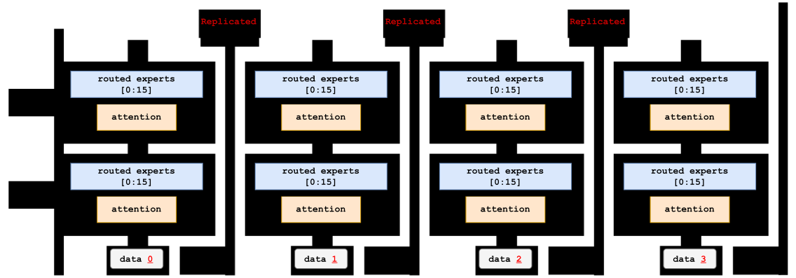
Start with replicated data parallelism and no model parallelism. Let \(D\) denote the DDP degree. Every rank holds the complete model (Figure 6), processes different training examples, and accumulates gradients for corresponding parameters. Before an optimizer update, a collective reduction produces the same synchronized gradient for each replicated parameter, so all replicas apply the same update and stay identical. This is the standard replicated-data-parallel contract implemented by PyTorch DDP (Li et al. 2020). As in Section 3, static refers to placement, not to persistent memory: the weights stay at stable GPU locations, and the optimizer still updates their values after every successful step.

FSDP uses a different parameter-materialization policy for data parallelism. Persistent parameter, gradient, and optimizer-state allocations are sharded across the FSDP group. Before a wrapped unit—for example, one Transformer block—runs its forward or backward computation, FSDP gathers that unit’s complete weights. After the computation consumes those weights, FSDP frees the gathered copy and keeps only the local shard; backward also reduce-scatters gradients into their persistent shards. FSDP thereby lowers persistent parameter, gradient, and optimizer memory at the price of gathering and materializing weights around each layer use. Both methods still process different input data. They differ in which complete weights remain materialized between uses. The original FSDP paper and the current FSDP2 documentation define this mechanism and its reshard policies (Zhao et al. 2023; PyTorch Contributors 2026e).

Mixed-precision training separates the representation used by model computation from the higher-precision values used by the optimizer (Micikevicius et al. 2018). The following terms distinguish the three parameter-sized allocations used throughout this section.

Figure 6Interactive · conceptual, no measured quantities

Different data on every GPU, one synchronized update

Step

1Step 1: Different data2Step 2: Local gradients3Step 3: Synchronize4Step 4: Same update

Step 1 of 4 · Different data

“Every rank holds the complete model … processes different training examples …”

DP = 4, as in the report figure. Hues mark which input produced each local gradient. Point at, tap, or tab to a part (arrow keys move between parts) to read the report’s description; tap it again, tap outside, or press Escape to return to the step.

Figure 6. A four-GPU DDP example with no model-parallel sharding. With DP\({}=4\), every GPU holds a static replica of the same attention layers and complete routed-expert pool, experts \(0\)–\(15\), while processing different input data. DDP synchronizes the gradients of these replicated weights; it does not itself shard the model shown here.

These dtypes are training-recipe choices, not requirements imposed by DDP or optimizer sharding. DeepSeek-V3 and Megatron-Core report storing both AdamW moments in BF16 while retaining FP32 main weights and accumulated gradients (DeepSeek-AI et al. 2024; Yan et al. 2026). Olmo keeps both AdamW moments in FP32 in the configurations described here; we have not evaluated lower-precision moment storage in this stack.

Let \(B\) be the tokens processed by one rank in an optimizer step, \(m\) the number of microbatches, \(K\) the number of active experts, \(d\) the model width, and \(D\) the DDP degree. Table 4 gives approximate resource costs for the work introduced in Section 1.3. The table omits constant factors and hardware efficiency.

These proportionalities identify pressure points; they are not additive terms in an elapsed-time model. Collective traffic also depends on the algorithm, topology, and overlap with other work. For example, ring all-reduce moves approximately \(2(D-1)/D\) payload copies per rank, while aggregate network traffic additionally grows with the number of ranks (Patarasuk and Yuan 2009).

The capacity-to-active gap is especially clear for the expert MLP. A bias-free SwiGLU expert pool with model width \(d\), expert intermediate width \(h_e\), and \(N\) routed experts stores approximately \(3Ndh_e\) parameters, whereas one token evaluates approximately \(3Kdh_e\) of them. Parameter-sized work can therefore grow with \(N\) while useful expert compute grows with \(K\). The next subsection compares how often DDP and FSDP perform that parameter-sized work.

4.2 FSDP Gathers per Microbatch; DDP Synchronizes per Global Step

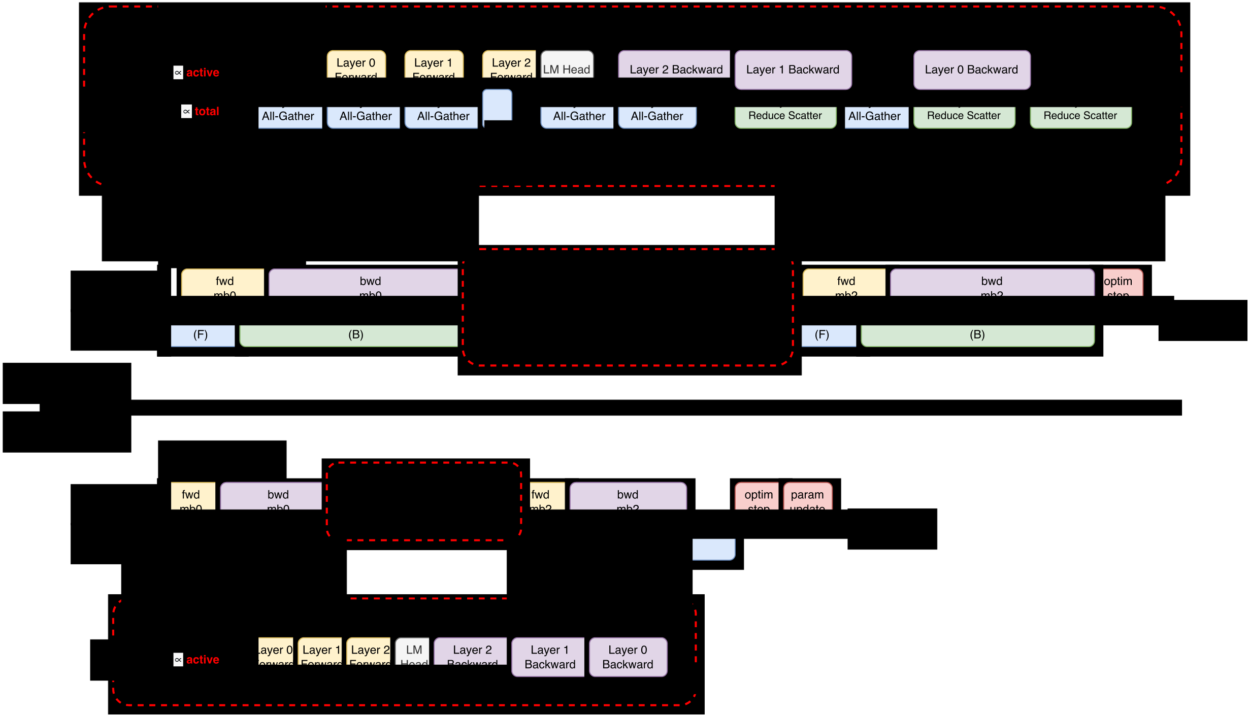
An optimizer step is the complete accumulation window that produces one model update. Suppose it contains \(m\) microbatches of \(b\) tokens per rank, so the rank-local accumulated batch is \(B=mb\). At fixed microbatch shape, useful model work grows the same way under either data-parallel choice: \[ W_{\mathrm{useful}}(m) \propto mbP_{\mathrm{active}}. \tag{7} \] The parameter-sized communication differs between the two alternatives (Figure 7):

• With DDP, gradient synchronization and, when using a distributed optimizer, compute-weight reconstruction occur once per optimizer step. Their payload scales with the rank-local parameter count, \(W_{\mathrm{DDP\ boundary}}\propto P_{\mathrm{local}}\).

• With FSDP, weight gathering and freeing recur as each wrapped unit is used in every microbatch. Across the accumulation window, this movement scales as \(W_{\mathrm{FSDP\ materialization}}\propto mP_{\mathrm{local}}\).

The DDP and FSDP terms describe alternative designs; they are not paid together. Increasing \(m\) spreads DDP’s once-per-step synchronization over more useful work, whereas it repeats FSDP’s weight movement. The optimizer update itself remains once per optimizer step in both designs.

On the Olmo-core DDP path, non-final microbatches run under no_sync() (Li et al. 2020). Gradients accumulate in stable buffers, and the complete window ends with one ordered sweep of bucketed all-reduces. When the distributed optimizer is enabled, it then updates each rank’s FP32 main-weight and optimizer-state shards and reconstructs the compute weights once. Replica synchronization therefore occurs at the global-step boundary, even with optimizer sharding.

With FSDP, each wrapped unit must instead be materialized for its forward and backward computation and freed after each use. Gradient accumulation can delay the optimizer step, but it does not eliminate this repeated weight movement. Retaining every gathered unit across the accumulation window instead trades that movement for higher memory, as discussed in Appendix B.3 (PyTorch Contributors 2026e).

Figure 7Interactive · illustrative, schematic phase widths from one profile · not a benchmark

Scrub one optimizer step: when does each design move parameters?

View

One optimizer stepInside one microbatch

Microbatches m

3 · as drawn

• Forward
• Backward
• All-gather (weights)
• All-gather + reduce-scatter
• Gradient reduction
• Optimizer

Full-reshard FSDP

Compute

bwd mb1

Communication

All-Gather + Reduce-Scatter (B)

Collective phases started

4 of 6 (2 per microbatch)

Olmo-core DDP

Compute

bwd mb2

Communication

grad reduce

Gradient synchronizations started

1 of 1 (per optimizer step)

Useful work (Equation 7)3 microbatches∝ mbP_active

FSDP weight movement6 collective phases∝ mP_local · grows with m

DDP synchronization1 gradient reduction∝ P_local · once per step

“Increasing m spreads DDP’s once-per-step synchronization over more useful work, whereas it repeats FSDP’s weight movement.”

Box widths are read from the report figure’s editable source; with m ≠ 3 the drawn microbatch pattern is repeated. The no_sync() spans, the Weights lane and the “Full weights present” lanes are web additions, derived from the Section 4.2 text and the drawn phases (a layer’s full weights exist from the start of its all-gather until the computation that uses them ends); the report figure does not draw them. Hover, tap, drag, or use the arrow keys to move the playhead.

Figure 7. Weight materialization and gradient synchronization run on different clocks. Under the illustrated FSDP schedule, unsharded weights are materialized around layer use in each microbatch. DDP instead uses static replicas of its local weights throughout the accumulation window and synchronizes accumulated gradients at the optimizer-step boundary. When EP is enabled, token dispatch and combine still recur in every routed layer and microbatch. The phase widths were manually reconstructed from one representative profile and preserve its approximate timing proportions; the diagram is not an aggregate benchmark.

DDP moves gradient reduction and optimizer reconstruction to the global-step boundary, but it does not make all communication independent of \(m\). Once EP is enabled, dispatch and combine move routed token rows, and their backward adjoints, in every routed layer and microbatch. Accumulating more microbatches spreads the once-per-step gradient synchronization and optimizer update over more useful work, but it does not reduce each microbatch’s EP traffic or enlarge its grouped-GEMM shapes.

The preliminary single-node accumulation sweep in Figure 8a shows the expected global-batch signature without mixing in EP. It fixes the model at 48 routed experts, approximately 3.2B active and 19B total parameters, fixes the rank-microbatch shape, and changes only the number of accumulated microbatches. Both paths run with EP disabled.

Figure 8 places this accumulation result beside the model-size sweep used in the next subsection. The panels test different questions: the left varies how much useful work shares one synchronization boundary, while the right varies how many inactive expert parameters the system must store and manage.

Figure 8Interactive · measured, preliminary · one 8×B300 node, eight-layer BF16 model

Two sweeps, two limits: batch size and expert parameter size

aAccumulation amortizes DDP’s per-step synchronization.

x-axis

DoublingLinear

• DDP (no EP)
• FSDP

Global batch 4 Mi tokens · 48 routed experts · EP off

DDP (no EP)41.4%+16.2 pts since 128 Ki

FSDP29.8%+3.4 pts since 128 Ki

DDP − FSDP+11.6percentage points

bEP delays DDP’s expert-capacity memory wall.

• MoE DDP + EP8
• MoE DDP + EP1
• MoE FSDP
• Dense references (3.2B)

N = 128 routed experts · 47B total · 3.2B active · top-4

DDP + EP842.1%52.0K tokens/s/GPU

DDP + EP1OOMout of memory

FSDP15.7%19.4K tokens/s/GPU

Top-4 random routing, no PP, one run per point. Plotted from the report’s measurement table, the same rows as the original panels; values are printed to one decimal as in the report figure, and differences are computed from them. Tokens/s/GPU appear where the table records them. Hover, tap, or use the arrow keys on a chart to read every point; legend buttons hide or show a series.

Figure 8. Global-batch and model-size sweeps expose different limits. Preliminary single-node measurements use eight B300 GPUs, an eight-layer BF16 MoE model, top-4 random routing, no PP, and approximately 3.2B active parameters. Left: with EP disabled and 48 routed experts (19B total parameters), DDP useful-model FLOPs utilization (MFU) rises from 25.2% to 41.4% between 128-Ki and 4-Mi-token global batches (\(1\ \mathrm{Ki}=2^{10}\) and \(1\ \mathrm{Mi}=2^{20}\) tokens), while FSDP rises from 26.4% to 29.8%. Right: total parameters grow from 4.6B to 47B; no-EP DDP runs out of memory at 64 and 128 experts, no-EP FSDP continues to fit but loses useful-model MFU, and DDP+EP8 remains nearly flat. Each point is one run, so the curves show preliminary scaling behavior rather than run-to-run variance. They do not decompose peak memory or attribute the trend to a specific communication phase.

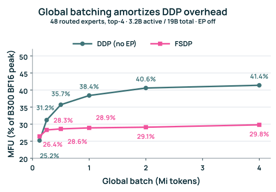
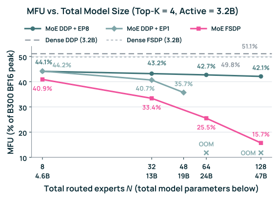
These trends are consistent with the cost model: DDP spreads its once-per-step work over more useful computation as the batch grows, while FSDP repeats its weight gathering in every microbatch. Each point is a single run without a matched communication profile, so the figure shows the trend but not its exact cause, and it measures throughput, not training quality or time to a target loss.

4.3 DDP Alone Hits a Memory Wall

Static replicas require a local partition that fits in memory. DDP removes repeated weight materialization only by keeping its compute weights and selected training buffers present throughout the accumulation window. Peak memory therefore combines persistent training state with execution working memory, summarized in Table 5.

FSDP has a direct advantage in persistent training-state memory. With enough shard ranks, it can make each rank’s long-lived parameter, gradient, and optimizer-state contribution small, although the currently materialized unit, activations, and temporary buffers still contribute to peak memory. DDP keeps the compute-weight representation of its rank-local partition complete. That partition, its gradient buffers, and the execution working set must all fit at once.

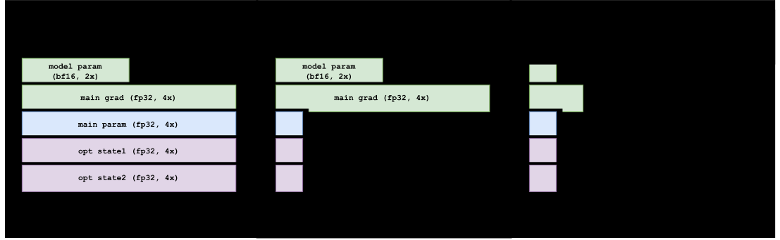
Figure 9 isolates the parameter-sized persistent training-state allocations directly changed by the distributed optimizer and EP under one concrete policy.

Figure 9Interactive · conceptual, per-parameter byte accounting · not measured memory

Choose D and M_E: what does one parameter cost each rank?

Replica ranks D

8

EP-MP degree M_E

1248

• Compute weight BF16 · 2 B
• Gradient buffer FP32 · 4 B
• Main weight FP32 · 4 B
• Optimizer state 1 FP32 moment · 4 B
• Optimizer state 2 FP32 moment · 4 B
• Weight + gradient floor

DDP18 Bper parameter, every rank

+ distributed optimizer7.5 B41.7% of naive DDP

+ EP · routed-expert parameter3 B16.7% of naive DDP

EP row as ranks · D = M_E × D_E = 4 × 2

Point at, tap, or tab to a rank: its card holds the copies of one expert shard; one rank from each card forms an EP-MP group.

Shard 11/4 of experts

2 copies

Shard 21/4 of experts

2 copies

Shard 31/4 of experts

2 copies

Shard 41/4 of experts

2 copies

“Because the original data-parallel group has size D = M_ED_E, expert optimizer state is still divided across the same total degree D after the two stages of sharding.”

“The mechanism recovers much of the optimizer-state memory that motivated FSDP without evicting or rematerializing compute weights between microbatches, but it does not remove the replicated weight and gradient floor.”

The figure’s settings are the default (D = 8; M_E = 4, D_E = 2); other values evaluate the same expressions with even sharding. The bottom row applies to routed-expert parameters. Dashed marks show the weight and gradient floor that the distributed optimizer leaves unsharded. Tap a bar segment or a legend entry to highlight one component.

Figure 9. The distributed optimizer and EP reduce different parts of DDP’s persistent parameter-sized training state. Under the illustrated BF16-execution, FP32-gradient, and two-moment FP32 optimizer policy, naive DDP uses 18 bytes per parameter. Sharding the FP32 main weights and optimizer states evenly over \(D\) replica ranks reduces this to \(6+12/D\) bytes while compute weights and gradient buffers remain replicated. Sharding routed-expert compute weights and gradients over the expert-parallel model-sharding degree \(M_E\) (EP-MP; defined in Section 5) further reduces their per-rank memory contribution to \(6/M_E+12/D\) bytes when \(D=M_ED_E\). Dense and shared parameters follow their separate replica groups. This accounting excludes execution working memory, including activations, routing and communication buffers, kernel workspaces, execution caches, and allocator fragmentation, as well as uneven shards and small auxiliary tensors that are not sharded.

The model-size sweep in Figure 8b makes the wall visible while holding useful expert work approximately fixed. Top-\(K\) stays at 4 and the active model size near 3.2B parameters as the routed-expert pool grows from 8 to 128 experts. DDP without EP fits at 8, 32, and 48 experts, then runs out of memory at 64 and 128. FSDP without EP continues to fit, but its measured MFU falls as total parameter size grows. DDP+EP8, which also shards the routed-expert pool across eight ranks, remains near 42–44% MFU over its measured points.

In the right panel, DDP+EP8 stores one eighth of the routed-expert pool per EP-MP shard; the dashed dense references were measured separately. Its measured MFU is nearly flat, but the per-rank expert shard still grows as \(N/8\). This residual growth matters more as modern MoE designs increase \(N\) while keeping \(K\) small (Table 1): EP changes the per-rank growth from \(N\) to \(N/M_E\), but it does not make memory independent of total expert parameter size. Olmo therefore reduces the rank-local partition with a distributed optimizer, EP, and PP.

4.3.1 Distributed Optimizer Shards FP32 Main Weights and Optimizer States

The first of these three mechanisms, the distributed optimizer, keeps model execution unchanged while shrinking the memory for FP32 main weights and optimizer states. Under the illustrated AdamW-like policy, one parameter contributes a 2-byte BF16 compute weight, a 4-byte FP32 gradient-accumulation slot, a 4-byte FP32 main weight, and two 4-byte FP32 moments. Naive DDP therefore carries 18 bytes per parameter before execution working memory. The distributed optimizer leaves the compute weight and gradient buffer replicated within that parameter’s replica group, but shards eligible FP32 main weights and optimizer states over the group. The idealized \(6+12/D\) expression in Figure 9 assumes even sharding. This optimizer-state partition follows the design family introduced by ZeRO (Rajbhandari et al. 2020).

Figure 10 compares the two useful balanced layouts with a naive baseline. Concatenate-then-shard flattens all eligible optimizer-state tensors into one sequence and partitions that sequence across ranks. It balances the aggregate optimizer state and does not require every tensor to be individually divisible by the sharding degree. Its cost is bookkeeping: shard boundaries may cut through tensors, so optimization, weight reconstruction, and checkpointing must all preserve a global map from each tensor to its flat-buffer views and offsets.¹ The figure’s same-param-count baseline assigns the same number of complete parameter tensors to every rank. It does not equalize the number of scalar elements. Because tensor sizes vary widely, equal tensor counts can produce severely unequal byte counts and are the least useful of the three layouts.

Figure 10Interactive · conceptual layout, illustrative tensor sizes

Shard the same four tensors three ways

Layout

Concatenate-then-shardSame param countPer-tensor · Olmo

Replica group D

234figure78

• param 0
• param 1
• param 2
• param 3

Largest rank holds1601.00× the even share of 160

Tensors cut across ranks4 of 4each sharded tensor is cut 4 ways

Replicated on every rank0all divisible by D

Index bookkeepingPer tensorlocal to each tensor

“Olmo instead divides each eligible main-weight and optimizer-state tensor independently into D equal contiguous shards.”

Tensor sizes are the figure’s drawn bar widths (illustrative units). Dashed marks on the tensor bar show where this layout cuts; the dashed vertical line marks an even share. The per-tensor rule shards a tensor only when its element count divides by D (the report’s policy also requires it to be sufficiently large; all four count as large here), so with D = 3 or 7 the illustrative sizes stop dividing evenly. Tap a tensor or its name to follow it across ranks.

Figure 10. Optimizer-state layout choices. Colors identify eligible FP32 optimizer-state tensors associated with different model parameters; they do not represent the replicated BF16 compute weights. Dashed lines mark the ranges assigned to each rank in an optimizer replica group of size \(D=4\). Concatenate-then-shard balances the flattened optimizer state globally but requires explicit view and offset metadata. The same-param-count baseline preserves whole tensors but can severely imbalance bytes. Olmo instead divides each eligible main-weight and optimizer-state tensor independently into \(D\) equal contiguous shards.

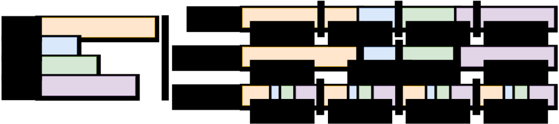
Olmo uses the per-tensor layout in the bottom row. Each eligible tensor is flattened and divided independently across its optimizer replica group; its FP32 main weight and optimizer states use the same rank-local slice. The mapping is local to one tensor, so update, reconstruction, and checkpoint views remain direct and easy to inspect. The trade-off is that the current policy shards a tensor only when it is sufficiently large and its element count is divisible by the replica-group size. Small or non-divisible optimizer-state tensors remain replicated, as do scalar step counters. This fallback does not prevent training, but it reduces the memory saved by the distributed optimizer.

In practice, this restriction is mild for the regular, mostly power-of-two replica groups in our production configurations, including groups of 128 ranks: nearly all large model tensors are divisible by these group sizes. Irregular sharding degrees such as 7 or 13 would cause more tensors to remain replicated, but we have not encountered that case in our production runs. Muon changes the number of optimizer history tensors, not this placement rule.

At the end of the accumulation window, DDP first produces reduced FP32 gradients. Each rank narrows the relevant gradient into the shard corresponding to its FP32 main-weight shard, updates that shard and its optimizer states locally, and then participates in coalesced all-gathers that reconstruct the updated compute weights. Thus gradient reduction, sharded update, and reconstruction happen once per optimizer step. The mechanism recovers much of the optimizer-state memory that motivated FSDP without evicting or rematerializing compute weights between microbatches, but it does not remove the replicated weight and gradient floor.

4.3.2 EP Shards Expert Weights and Gradients

The second mechanism reduces the routed-expert memory that the distributed optimizer leaves replicated. With EP-MP degree \(M_E\), each rank stores roughly \(N/M_E\) routed experts and their gradient buffers rather than all \(N\) experts. Ranks holding copies of the same expert shard form an EP-DP group of size \(D_E\): they reduce that shard’s gradients together, and the distributed optimizer shards its FP32 main weights and optimizer states over those \(D_E\) replicas. Because the original data-parallel group has size \(D=M_ED_E\), expert optimizer state is still divided across the same total degree \(D\) after the two stages of sharding. EP’s additional memory saving is therefore in compute weights and gradient buffers; it is not another factor applied to optimizer state that was already sharded over \(D\). Section 5 introduces the EP-MP and EP-DP topology and the dispatch/combine traffic paid for this saving.

4.3.3 PP Shards Layers and Their Persistent Training State

EP divides the expert pool inside a layer, but every rank may still hold too many layers, dense weights, shared experts, and activations. PP assigns different layer ranges and their weights, gradient buffers, and optimizer shards to different stages, reducing this persistent training-state memory in each rank-local partition. It introduces a different tax: activation transfers, pipeline bubbles, and multiple in-flight microbatches. Section 6 develops those schedules and memory trade-offs. Together, the distributed optimizer, EP, and PP make DDP practical at model sizes where ordinary replicated DDP is not.

4.4 Olmo-Owned DDP

The Olmo-core DDP training stack includes both replica synchronization and the update path around it. PyTorch’s standard DistributedDataParallel wrapper is designed around one process group and ordinary Parameter.grad handling (Li et al. 2020; PyTorch Contributors 2026d). Olmo combines separate execution and update precision, parameter-specific replica groups after EP, sharded optimizer states, derived MXFP8 representations, and explicit completion after gradient accumulation or a pipeline schedule. Each piece can be assembled from PyTorch mechanisms, but operating them as one coordinated update path requires integration deep enough that Olmo implements and controls the DDP path directly rather than layering it around the standard wrapper.

4.4.1 Hybrid Precision Control

Execution precision and update precision serve different goals. BF16 and MXFP8 reduce model execution and storage cost. Gradient accumulation sums contributions across microbatches, gradient reduction combines ranks, and the optimizer integrates updates over many steps. Mixed-precision training keeps an FP32 master copy of the weights for updates and performs large sums in FP32 (Micikevicius et al. 2018); we apply the same principle to gradient accumulation and reduction. In the Olmo-core DDP configuration described here, model execution uses BF16 or selected MXFP8 paths, while normal parameter gradients accumulate in dedicated FP32 bucket views, reduce in FP32, and feed FP32 main weights and optimizer states.

This separation is more specific than generic mixed-precision execution. For an ordinary BF16 parameter, autograd’s leaf AccumulateGrad node first produces a temporary BF16 param.grad. A post-accumulate hook immediately adds that gradient into the parameter’s FP32 accumulation buffer and clears param.grad. Each FP32 accumulation buffer is a view into a flat bucket built before training, and gradient reduction operates directly on that bucket.² The policy described here uses FP32 accumulation and FP32 reduction. After the optimizer updates an FP32 main weight, the BF16 or MXFP8 compute-weight representation is refreshed. MXFP8 weight stores use the optimizer-integrated path described below.

4.4.2 EP Requires Multiple DDP Groups

EP makes a single process group insufficient for one model part. Dense parameters are replicated across the dense data-parallel group. Ranks along EP-MP hold different expert shards and must not average those shards together; only EP-DP ranks holding copies of the same expert shard reduce its gradient. A single standard PyTorch DDP wrapper selects one process group for all of its parameters, whereas the MoE model part contains both kinds of parameter.

For parameters handled by the bucketed DDP path, Olmo chooses a replica group per parameter and forms buckets only among parameters with compatible groups and storage and communication dtypes. Non-final microbatches accumulate locally. Explicit finalization launches the remaining bucket reductions in a stable order and preserves gradients from experts that appeared earlier in the window but not in its final microbatch. Section 5 derives the topology that these groups implement.³

4.4.3 Native MXFP8 Integration

An MXFP8 compute-weight cache is not independently updated. The FP32 main weight is the source used to rebuild the derived, orientation-specific MXFP8 caches for forward and dgrad. After an update, the optimizer gathers any sharded FP32 main weight, reconstructs the full weight, and refreshes the caches coherently. The current path casts through a BF16 compute-weight representation before quantization, so we describe the caches as derived from the FP32 main weight rather than as a direct FP32-to-MXFP8 conversion. Section 11 covers formats, scales, and kernels, together with the cache formats and refresh points.

4.4.4 Collectives and Weight Reconstruction Stay Outside the Compiled Update

Olmo keeps collective launches and compute-weight reconstruction outside the compiled optimizer computation. This separates local shard updates from the communication and refresh phases that surround them, making their order explicit and keeping each phase visible in the step timeline. The same update path coordinates gradient clipping with the optimizer step and performs per-group initialization checks.

4.5 DDP and FSDP Optimize Different Bottlenecks

FSDP minimizes long-lived unsharded parameter storage by materializing weights around use. Olmo-core DDP keeps its rank-local compute-weight partition, which must fit in memory, materialized at stable locations across accumulation and moves gradient synchronization and optimizer reconstruction to the global-step boundary. The distributed optimizer lowers FP32 main-weight and optimizer-state memory, EP divides the routed-expert pool, and PP divides layers. Olmo’s implementation integrates the precision, replica-group, and derived-representation refresh rules needed by that composition.

Dense Olmo continues to use FSDP/HSDP. When useful compute grows with materialized parameters or peak parameter, gradient, and optimizer memory is the primary constraint, FSDP or HSDP remains an effective foundation. The current single-node sweeps establish two local scaling patterns in the eight-layer model: accumulation amortizes more of DDP’s step-boundary work, and increasing expert parameter size raises pressure on an unsharded local partition. They do not establish a universal sparsity crossover, optimization quality, or time to a target loss.

The next section develops EP as the model-parallel mechanism that makes the routed-expert partition fit. It explains which ranks hold different expert shards, which ranks hold replicas of the same shard, and why saving weight and gradient memory introduces dispatch and combine on the microbatch clock.