Section 01: Why the Dense Training Assumptions Break

1.1 Mixture of Experts (MoE): Sparse Activation

MoE separates total and active parameters. In a dense Transformer block (Vaswani et al. 2017), every token—one position in the input sequence—is processed by the same feed-forward network (FFN). Making that FFN larger gives the model more capacity and increases computation for every token. MoE adds parameters while using only a subset of them for each token.

Each token selects a few experts. The router scores the \(N\) available experts and chooses the top \(K\). The runtime sends—or dispatches—the token’s vector to those selected experts. Each selected expert applies its FFN to the vector. The router supplies a combination weight for each selected expert, and the combine operation multiplies the expert outputs by those weights, sums them, and restores the result to the token’s original sequence position. The router and experts learn together with the rest of the model. This sparse-gated pattern was established by early large-scale MoE work and later simplified by the Switch Transformer (Shazeer et al. 2017; Fedus et al. 2022).

For token representation \(x_t\), let \(S_t\) be the selected expert set, let \(p_{t,e}\) be expert \(e\)’s combination weight, and let \(f_e\) be that expert’s FFN. Then

\[ y_t^{\mathrm{routed}} = \sum_{e \in S_t} p_{t,e} f_e(x_t), \qquad |S_t|=K \ll N. \tag{1} \]

Some MoE blocks also include a shared expert, an FFN that every token uses alongside its selected routed experts. Attention, embeddings, normalization, the router, and any shared expert also remain active when most routed experts do not. And because the router’s choices depend on the input, experts do not necessarily receive equal numbers of tokens. Training systems use load-balancing objectives and capacity limits to keep one expert from becoming an unbounded hotspot (Shazeer et al. 2017; Fedus et al. 2022; Dai et al. 2024).

Consider a layer with \(N=128\) routed experts and \(K=4\). The model has 128 routed expert FFNs, yet a single token uses only four of them. We therefore distinguish the model’s total parameter count from the number of parameters active for one token.

This per-token accounting only approximates total model FLOPs, because attention, routing, shared branches, and auxiliary work also contribute. Sparse activation still allows substantially more parameters without a proportional increase in per-token computation. Different token paths may also encourage experts to learn different functions, although useful specialization is neither guaranteed nor assigned by hand.

Models are getting larger—and sparser. A visible design trend among recent high-capacity MoEs is to grow total expert parameter size faster than the active parameter count. The cleanest evidence comes from comparisons within one model family: from DeepSeek-V3 to DeepSeek-V4-Pro, and from Qwen3-235B-A22B to Qwen3.5-397B-A17B, total parameters grow substantially while the active count grows far less or even falls, so the advertised parameter activation ratio drops (DeepSeek-AI et al. 2024, 2026; Yang et al. 2025; Qwen Team 2026b).

Table 1 places those examples among their contemporaries. It is deliberately a design survey rather than a leaderboard: model objectives, layer types, and parameter-counting conventions differ, and neither activation ratio alone measures end-to-end efficiency.

For the routed language models they study, Clark et al. (2022) show that total parameter count and per-token computation form distinct scaling axes. Fitted scaling laws for fine-grained MoEs further predict that compute-optimal MoE configurations reach lower validation loss than dense Transformers at the same training-FLOP budget, with the predicted advantage widening at larger budgets (Ludziejewski et al. 2024). Yet more sparsity is not automatically better: the best sparsity level depends on constraints such as total parameter count and training compute (Abnar et al. 2025). These results indicate that well-configured MoEs can improve the compute–quality frontier, although a given MoE need not beat a dense model at matched FLOPs.

1.2 Lower FLOPs Do Not Guarantee Lower Wall Time

Useful model FLOPs account for arithmetic but leave out much of the work required to train an MoE. The training system must also move weights and token activations, synchronize ranks, and absorb load imbalance. Those costs determine how many GPU-hours it actually takes to reach the desired quality.

Let \(F\) be the useful model FLOPs needed to reach a declared training or quality target, \(R\) the realized throughput in useful model FLOPs per GPU-hour under the same accounting convention, and \(H\) the GPU-hours consumed. We compare the GPU-hours required by MoE with those required by dense training to reach the same target:

\[ \rho_H \equiv \frac{H_{\mathrm{MoE}}}{H_{\mathrm{dense}}} = \frac{F_{\mathrm{MoE}}}{F_{\mathrm{dense}}} \frac{R_{\mathrm{dense}}}{R_{\mathrm{MoE}}}. \tag{4} \]

Here \(\rho_H<1\) means MoE uses fewer GPU-hours than dense training; for example, \(\rho_H=0.5\) means half as many. For runs using the same number of GPUs, \(\rho_H\) is also the elapsed wall-time ratio.

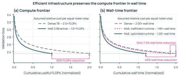
The first factor captures algorithmic efficiency: a smaller \(F_{\mathrm{MoE}}/F_{\mathrm{dense}}\) means fewer useful FLOPs are needed to reach the target. The scaling results above suggest that a well-configured MoE can reduce this factor in the regimes they study. The second factor captures the throughput penalty: when MoE sustains lower useful-FLOP throughput than dense training, \(R_{\mathrm{dense}}/R_{\mathrm{MoE}}>1\). This penalty can erase the algorithmic gain (Figure 3).

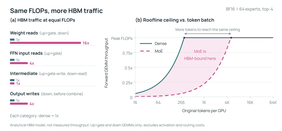
Equal FLOPs can require more HBM traffic. Compared with a dense FFN of equal active compute, an MoE reads more weights from high-bandwidth memory (HBM), each reused by fewer tokens. Materialized top-\(K\) routes also give grouped GEMM \(K\) input rows and \(K\) final output rows per original token; combine happens after those outputs are written. A roofline estimates the throughput ceiling imposed by arithmetic and HBM traffic (Austin et al. 2025). Figure 2 shows how the extra bytes lower MoE’s modeled ceiling at small batches, even before routing or communication time is added. More tokens per expert amortize the weight reads: both curves eventually reach the same compute ceiling. Appendix A.8 derives the comparison; Section 9.6 measures how actual kernel efficiency changes with rows per expert.

Figure 2Interactive · conceptual analytical model, no measured quantities

Scrub the token batch: where does MoE reach the same ceiling?

Original tokens per GPU

1,024

Beyond the report · routed experts N

163264report128

• Dense FFN, hidden width Kh
• MoE, N = 64 experts of width h, top-4
• MoE is HBM-bound here

(a) HBM traffic at equal FLOPs MoE / dense, per category

• Weight reads up+gate, down

  1×16×

• FFN input reads up+gate

  1×4×

• Intermediate up+gate write, down read

  1×1×

• Output writes down, before combine

  1×4×

Each category is normalized separately; the ratios do not add.

Bytes at 1,024 tokens one forward GEMM pair, common scale, computed from the model

Dense

520 MB

MoE

6.61 GB

• Weight reads
• FFN input reads
• Intermediate
• Output writes

MoE-to-dense bytes

12.7×

Rows per expert, TK/N

64

Dense GEMMs

up/gate compute‑bound · down compute‑bound

MoE GEMMs

up/gate HBM‑bound · down HBM‑bound

The report’s model: N = 64, K = 4, d = h = 4,096, BF16, balanced routes, one HBM read or write per operand or result, forward up/gate and down GEMMs only. Ceilings within that model, not measured rates; activation, packing, combine, network and backward costs are excluded (Appendix A.8). Byte totals are computed from the same equations; other N values explore them beyond the report.

Figure 2. Equal FLOPs do not imply equal HBM traffic. The forward fused up/gate and down GEMMs of a dense FFN with intermediate width \(Kh\) are compared with \(N\) experts of intermediate width \(h\), selecting \(K\) per token. Here \(N=64\), \(K=4\), and the model width and expert intermediate width are \(d=h=4096\). (a) GEMM-side HBM byte categories, each normalized separately to dense. These ratios are not additive: each category contributes according to its absolute byte volume, not equally. The intermediate row counts up/gate output writes and down input reads, excluding the pointwise activation’s own accesses. (b) Analytical ceilings in bfloat16 (BF16), normalized to peak FLOPs, with balanced routes and one HBM read/write per operand/result. Each curve adds the two GEMM times; pointwise activation, packing, combine, network, and backward costs are excluded. Conceptual illustration with no measured quantities; assumptions are detailed in Appendix A.8.

Model FLOPs utilization (MFU) reports useful model throughput as a fraction of a stated hardware peak (Chowdhery et al. 2023). Our complete-step results in Section 14 use the B300’s dense BF16 Tensor Core peak as a common denominator (NVIDIA 2026q), including for MXFP8 runs; those values are not utilization of the FP8 peak. Appendix B.11 gives the accounting.

An expert unused by one token contributes no expert compute for that token, but its parameters and optimizer states still consume memory. Depending on the parallelization method, gradient reduction and weight synchronization can also scale with total expert parameter size. Expert placement determines how far a routed token must travel. Routing itself adds work: count assignments, enforce capacity, move or permute token rows, run experts on the devices that store them, restore token order, and cope with imbalance. Useful model-FLOP accounting excludes most of this work.

Figure 3Interactive · illustrative simulated loss traces and assumed costs, not measured

Same loss curve, different clock: change only the runtime cost

Report cases

Inefficient infrastructure1.85×Optimized infrastructure1.20×

MoE wall-time cost per equal-token step (dense = 2)

1.85×

ρ_H = F_MoEF_dense × R_denseR_MoE = 0.50 × 1.85 = 0.925

MoE needs 92.5% of the dense GPU-hours: a 1.08× time-to-target advantage.

All MoE curves in (b) reuse the same simulated loss samples; only the cost per step changes the horizontal axis. The ratio follows Equation 4: equal-token steps make F_MoE/F_dense = 1/2 here, and the throughput penalty equals the MoE wall-time cost per step. All costs and curves are the report’s illustrative assumptions, not measurements or predictions for an Olmo run.

Figure 3. A FLOP advantage can shrink or survive in wall time. This illustrative, simplified comparison uses two power-law-shaped loss traces that run for 10,000 equal-token steps and end at the same loss. Panel (a) assigns the 3.5B-active/13B-total MoE a normalized useful-FLOP cost of \(1\) per step, versus \(2\) for the 7B dense model. Panel (b) maps the same MoE loss samples onto two hypothetical runtimes: normalized wall-time costs of \(1.85\) for inefficient infrastructure and \(1.2\) for optimized infrastructure, versus \(2\) for dense. The corresponding time-to-target advantages are only \(2/1.85\approx1.08\times\) and \(2/1.2\approx1.67\times\). All costs and loss curves are illustrative assumptions, not measurements or predictions for an Olmo run.

We observed low realized throughput in two early development baselines. One used a straightforward MoE configuration in Megatron-LM, NVIDIA’s distributed Transformer training framework (Shoeybi et al. 2019).¹ The other used the legacy MoE path in Olmo-core, Ai2’s training library for the Olmo model family; that path inherited fully sharded data parallel (FSDP), the parameter-sharding mechanism used for dense Olmo 3 training (Team Olmo et al. 2025) and described in Section 4. Both suggested that low realized throughput could consume much of the advantage predicted by active-FLOP accounting.

A controlled eight-layer experiment reproduces the Olmo-side slowdown. Figure 4 holds top-\(K\) and active size nearly fixed while increasing total routed-expert parameter size.² The legacy FSDP-based path loses throughput as total parameter size grows, even though useful expert compute per token stays nearly constant. The new distributed data parallel (DDP; Section 4) path with expert parallelism (EP; Section 5) degree 8 retains most of its dense throughput across the same parameter-size range. Active-FLOP accounting alone does not predict this difference.

Figure 4Interactive · measured, preliminary · one 8×B300 node, eight-layer BF16 model

Add experts at fixed active size: which path keeps its throughput?

Plot

Tokens/s/GPU% of own dense baseline

• Dense (old)
• MoE (old) · FSDP, no EP
• Dense (new)
• MoE (new) · DDP, EP8

MoE · 3.2B active of 47B total · N = 128, top-4

Old path · FSDP19.4K31.8% of its dense 61.0K

New path · DDP + EP852.0K82.5% of its dense 63.0K

Ratio of the two bars: 2.68×

Plotted from the report’s measurement table, the same rows as the original figure. Percentages are computed from those values. This is a composed-system comparison, not an isolated FSDP-versus-DDP or EP ablation; MoE runs use random routing (see the note in the text).

Figure 4. Throughput as total expert parameter size grows at nearly fixed active FLOPs. These preliminary measurements use an eight-layer bfloat16 (BF16) model on one 8\(\times\)B300 node without pipeline parallelism (PP; Section 6); MoE uses top-4 routing, and the new MoE path uses EP8. The old, dense-oriented FSDP path loses throughput as total expert parameter size grows, whereas the new DDP+EP path keeps MoE throughput within a modest margin of its dense baseline. This is a composed-system result, not an isolated FSDP-versus-DDP or EP ablation.

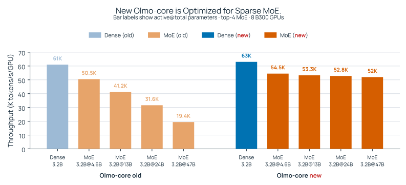
Figure 4 compares the old FSDP-based Olmo training stack with the new DDP+EP stack, changing several components together. It therefore does not isolate the benefit of DDP or EP alone, or rank Olmo against other training frameworks. It motivates the systems question pursued by this report: which costs continue to grow with total expert parameter size, and how the training stack can keep them from dominating wall time.

1.3 Sparse Routing Breaks the Dense Training Assumptions

Training cost includes useful model work and systems overhead. To organize the costs of an optimizer step, we use the following reference accounting:

\[ T_{\mathrm{step}} = T_{\mathrm{model}} + T_{\mathrm{tax}}. \tag{5} \]

Table 2 lists the work included in each term. \(T_{\mathrm{model}}\) is an ideal reference time for the prescribed forward and backward work at the hardware peaks for the precisions actually used, not the common BF16 normalization used for MFU. \(T_{\mathrm{tax}}\) is the remaining elapsed time, including execution below those peaks and exposed overhead. The table identifies sources of that overhead, not independent profiler durations to add together: communication and computation can overlap. Activation rematerialization, or recompute, discards selected forward activations and recomputes them for the backward pass instead of keeping them in memory. It adds executed FLOPs without increasing useful model FLOPs, and a recomputed routed block can also repeat dispatch and combine (Section 13). In a well-tuned dense stack, large, regular model computations usually keep these costs in a workable balance. In MoE, useful computation follows the active parameters, while much of the tax follows total parameter size or routed token assignments. Infrastructure built around dense assumptions can therefore let the tax dominate. The systems goal is to lower it until fewer useful FLOPs also mean less wall time.

1.3.1 Capacity Tax

Dense compute can amortize parameter-sized work. In a dense model, \(P_{\mathrm{active}}=P_{\mathrm{total}}\): adding parameters increases the forward and backward compute performed for every token as well as the parameters, gradients, and optimizer buffers that must be stored, reduced, or updated. The tax does not disappear, but it grows in step with useful model computation.

In MoE, the two no longer grow together. Sparse routing lets total expert parameter size grow while each token continues to execute only its selected experts. We call the following dimensionless ratio, compared at fixed token count, execution schedule, and hardware, the capacity-to-active gap:

\[ \Gamma_{\mathrm{capacity}} \ \equiv\ \frac{P_{\mathrm{total}}}{P_{\mathrm{active}}} = \frac{1}{\alpha_P}. \tag{6} \]

For dense models, \(\Gamma_{\mathrm{capacity}}=1\). For MoE, it can grow as new routed experts increase \(P_{\mathrm{total}}\) without proportionally increasing \(P_{\mathrm{active}}\). Related systems work observes the same decoupling between total model size and per-token work (Yan et al. 2026).

We call the concrete costs that continue to follow total parameter size the capacity tax. Weight and gradient storage, optimizer state, and some synchronization can grow without a matching increase in useful per-token compute. The ratio \(\Gamma_{\mathrm{capacity}}\) only measures how far stored parameters have outgrown the parameters each token uses; how much time that separation costs depends on the implementation. As the ratio increases, parameter-sized work grows relative to the useful computation available to amortize it.

Full-reshard FSDP matches dense models better than sparse MoE. Before model parallelism, ordinary DDP (Section 4) divides the training data while every rank stores the complete model. Adding DDP ranks therefore does not reduce per-GPU model memory. When a full dense-model replica no longer fits, dense Olmo uses FSDP to shard parameters, gradients, and optimizer state. In the full-reshard regime used by our comparison, FSDP all-gathers the full weights of each wrapped unit before the unit computes and frees them after each use (Zhao et al. 2023).³ For a dense model, the parameters materialized for a wrapped unit also support useful computation for every token. The materialization is still a tax, but a larger dense model brings a matching increase in useful model computation.

FSDP can make a large MoE fit as well, but its weight materialization no longer tracks useful work. In this configuration, every microbatch materializes the wrapped MoE unit’s parameter shards according to its stored expert parameter size, while useful expert compute follows the number of token–expert assignments. As \(P_{\mathrm{total}}/P_{\mathrm{active}}\) grows, weight movement can therefore grow without a proportional increase in useful model work. Full resharding solves the immediate fit problem, but its per-microbatch weight materialization becomes a substantial part of the MoE capacity tax.

Olmo uses DDP plus model parallelism for MoE. The Olmo MoE design composes DDP with two forms of model parallelism: EP (Section 5) shards the routed experts, and pipeline parallelism (PP; Section 6) assigns different layers to different stages. EP and PP first make each rank’s model partition small enough to fit; DDP then synchronizes replicas of that local partition. A distributed optimizer shards the larger FP32 main weights and optimizer states, while the compute weights—the BF16 or MXFP8 (Section 11) representations read by forward and backward—remain static across the accumulation window and are refreshed once per optimizer step. Section 3 introduces the broader parallelism toolbox before the following sections develop these choices.

1.3.2 Runtime Tax

Sparse execution adds work around the expert computation. For a fixed batch shape, a dense feed-forward layer executes a predictable sequence of large, regular operations. A routed MoE layer must first decide which experts will process each token. It must then arrange and move token rows to those experts, execute the selected experts, and restore and combine their outputs. This work repeats in every routed layer and every microbatch. Sparse execution requires this work, but it is overhead around the useful expert computation.

The extra time appears in several forms. Routing requires decisions, counting, and bookkeeping. Dispatch and combine add memory movement, permutations, and, when experts are distributed, communication. Expert computation can become less efficient when the routed batches are small or uneven. Dynamic shapes and load imbalance can also introduce temporary buffers, extra kernel launches, CPU overhead, synchronization, and contention between communication and computation. The exact mixture depends on the routing decisions, the runtime implementation, and the hardware.

We refer to these routing, compute-efficiency, and supporting runtime costs collectively as the MoE runtime tax. Unlike the capacity tax, it is not explained by model size alone: two batches with similar nominal model FLOPs can take different amounts of time because they route tokens differently and exercise the runtime differently. Section 5 examines token movement, Section 8 addresses host submission and synchronization, Section 9 studies expert compute efficiency, and Section 10 examines routing imbalance.

1.3.3 End-to-End Optimization

EP lowers the expert parameters stored and synchronized by each rank, but introduces token traffic. Recomputation lowers activation memory by repeating model work (Section 13). Reduced precision can speed up matrix multiplications and reduce communication volume, but adds conversion work and can expose launch overhead. Its numerical recipe also matters: with round-ceiling scaling, MXFP8 closely follows BF16’s loss and gradient-norm trajectories over our measured checkpoint-branched continuation (Section 11.3.5, Figure 56). Overlapping communication with computation shortens the step only when the slowdown it causes in the concurrent kernels is smaller than the communication time it hides (Section 5.9). These interactions are a recurring property of MoE systems (Yan et al. 2026). The report-wide matrix in Appendix D, Figure 76, summarizes the first-order benefits and costs of the parallelism, communication, scheduling, precision, runtime, and checkpoint methods developed in the rest of this report. We place the full matrix in the appendix because many of its columns are introduced only in later sections.

We therefore evaluate component changes by their effect on complete-step time and throughput for a given model, batch, and topology. An isolated kernel or collective speedup is insufficient to establish that effect.

The next section presents how these mechanisms are integrated into one end-to-end system: the Olmo-core DDP training stack.